Summary
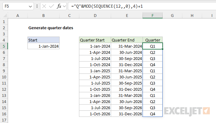
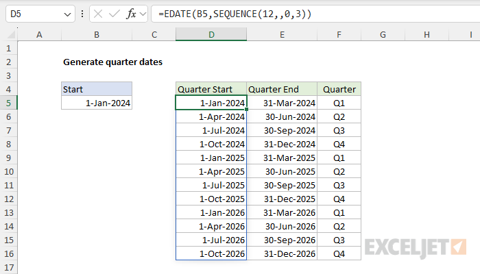
To generate a list of quarter dates, you can use the EDATE function with the SEQUENCE function. In the worksheet shown, the formula in D5 is:
=EDATE(B5,SEQUENCE(12,,0,3))
The result is a list of the next 12 quarter-start dates, beginning on the date in B5, which is January 1, 2024. The quarter-end dates in column E are based on a similar formula explained below.
Generic formula
=EDATE(A1,SEQUENCE(n,,0,3))
Explanation
In this example, the goal is to generate a list of quarter start and quarter end dates. This can be done by combining the SEQUENCE function with the EDATE and EOMONTH functions, as explained below.
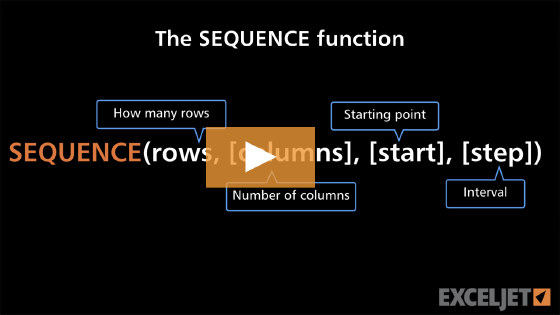
The SEQUENCE function
The SEQUENCE function generates a list of sequential numbers in an array. For example, the formula below generates a sequence of 5 numbers that begin with 1 and end with 5:
=SEQUENCE(5) // returns {1;2;3;4;5}
SEQUENCE has optional arguments for the start value and the step value. For example, if we provide zero as the start value, we get an array of 5 numbers that begin with zero and end with 4:
=SEQUENCE(5,,0) // returns {0;1;2;3;4}
If we provide 3 for the step argument, we get an array of numbers that begin with zero and end with 12:
=SEQUENCE(5,,0,3) // returns {0;3;6;9;12}
We use this behavior in the formulas below.
By default, SEQUENCE will generate data in rows. To generate data in columns, use the optional second argument, columns, and leave rows empty. For a brief overview, watch this video: The SEQUENCE function.
Quarter start dates
To create a list of quarter start dates, we use the EDATE function, which is designed to add months to a given start date. For example, if we use "1-Jan-2024" as the start date, we can create four quarter start dates by providing 0, 3, 6, and 9 to EDATE as the months argument:
=EDATE("1-Jan-2024",0) // returns 1-Jan-2024
=EDATE("1-Jan-2024",3) // returns 1-Apr-2024
=EDATE("1-Jan-2024",6) // returns 1-Jul-2024
=EDATE("1-Jan-2024",9) // returns 1-Oct-2024
The first formula does not change the date since the number of months is zero. The second formula adds 3 months, the third adds 6 months, and the fourth adds 9 months to the date. In all cases, EDATE returns the first of the month since the start date is also the first. In the worksheet shown, our goal is to generate a list of 12 quarter start dates beginning on January 1, 2024 (in cell B5). We do this by combining the EDATE function with the SEQUENCE function in a formula like this:
=EDATE(B5,SEQUENCE(12,,0,3))
Working from the inside out, the SEQUENCE function is configured to create a sequence of 12 numbers, starting at zero and incrementing by 3:
SEQUENCE(12,,0,3)
- rows - provided as 12 since we want 12 dates at the end
- columns - empty (defaults to 1)
- start - given as zero because we want to use begin on the start date
- step - given as 3 because we want to increment each number by 3
In this configuration, SEQUENCE returns an array of 12 numbers like this:
{0;3;6;9;12;15;18;21;24;27;30;33}
This array is passed directly to the EDATE function as the months argument.
=EDATE(B5,{0;3;6;9;12;15;18;21;24;27;30;33})
EDATE then returns 12 dates that begin with 1-Jan-2024 in an array like this:
{45292;45383;45474;45566;45658;45748;45839;45931;46023;46113;46204;46296}
The array is delivered to cell D5 and spills into the range D5:D16. These are Excel dates in their raw serial number format. Once the range is formatted with the number format "d-mmm-yyyy", the numbers will display the quarter start dates seen in the worksheet:
{"1-Jan-2024";"1-Apr-2024";"1-Jul-2024";"1-Oct-2024";"1-Jan-2025";"1-Apr-2025";"1-Jul-2025";"1-Oct-2025";"1-Jan-2026";"1-Apr-2026";"1-Jul-2026";"1-Oct-2026"}
Quarter end dates
To create a list of quarter-end dates, we use the EOMONTH function. EOMONTH works just like the EDATE function. However, instead of returning a date on the same day of the month, EOMONTH returns the last day of the month. For example, if we use "1-Jan-2024" as the start date, we can create four quarter-end dates by providing 2, 5, 8, and 11 to EOMONTH as the months argument:
=EOMONTH("1-Jan-2024",2) // returns 31-Mar-2024
=EOMONTH("1-Jan-2024",5) // returns 30-Jun-2024
=EOMONTH("1-Jan-2024",8) // returns 30-Sep-2024
=EOMONTH("1-Jan-2024",11) // returns 31-Dec-2024
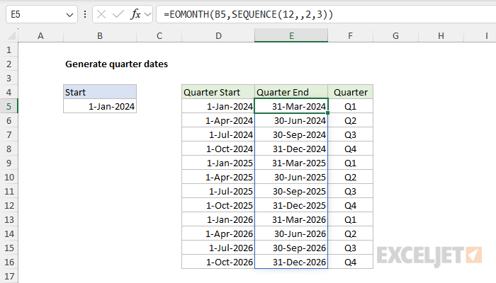
Notice that EOMONTH returns the last day of the month even though the start date is the first day of the month. In the worksheet shown, we want to list 12 quarter-end dates based on a start date of January 1, 2024 (in cell B5). We do this with EOMONTH and SEQUENCE like this:
=EOMONTH(B5,SEQUENCE(12,,2,3))
This formula is very similar to the EDATE + SEQUENCE formula we used to create quarter start dates above. The difference is that (1) we use the EOMONTH function instead of EDATE, and (2) we configure SEQUENCE in a slightly different way, starting the sequence at 2 instead of zero:
SEQUENCE(12,,2,3)
- rows - given as 12 because we want 12 dates
- columns - empty (defaults to 1)
- start - given as 2 to add 2 months to the start date
- step - given as 3 because we want to increment each date by 3 months
In this configuration, SEQUENCE returns an array of 12 numbers like this:
{2;5;8;11;14;17;20;23;26;29;32;35}
This array is returned directly to the EOMONTH function as the months argument:
=EOMONTH(B5,{2;5;8;11;14;17;20;23;26;29;32;35})
EOMONTH then returns 12 dates that begin with 31-Mar-2024 in an array like this:
{45382;45473;45565;45657;45747;45838;45930;46022;46112;46203;46295;46387}
The array is delivered to cell E5 and spills into the range E5:E16. When the number format "d-mmm-yyyy" is applied, the numbers will display the quarter-end dates seen in the worksheet:
{"31-Mar-2024";"30-Jun-2024";"30-Sep-2024";"31-Dec-2024";"31-Mar-2025";"30-Jun-2025";"30-Sep-2025";"31-Dec-2025";"31-Mar-2026";"30-Jun-2026";"30-Sep-2026";"31-Dec-2026"}
In the worksheet, the formula looks like this:
You might wonder if we can use the existing quarter start dates directly. Yes. Since we already have a list of quarter start dates in column D, another option is to use the EOMONTH function directly with the spill range like this:
=EOMONTH(+D5#,2)
This formula simply shifts each quarter's start date forward 2 months and returns the last day of that month. The result is exactly the same.
The plus sign (+) is needed before the spill range in this case. Without it, the formula will return a #VALUE! error. Some older functions, like EOMONTH, "resist" spilling when provided with a range. For example, EOMONTH(A1:A5,1) will return #VALUE even with valid dates in A1:A5. This limitation comes from certain functions expecting a single value instead of a range. The #VALUE! error is essentially reporting the range as an unexpected value. However, adding an operator in front of the reference will often fix the problem because it forces Excel to evaluate the expression first before the function runs. For an overview, see Dynamic Array Formulas in Excel.
Formula abbreviations
The quarter abbreviations seen in column F are generated with a formula like this in cell F5:
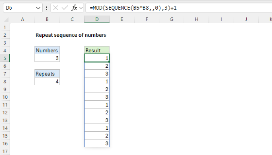
="Q"&MOD(SEQUENCE(12,,0),4)+1
At the core, this is a formula that repeats numeric sequences using the SEQUENCE function and the MOD function. We then concatenate a "Q" to the output. You can see the formula and result below: