Count specific characters in text string

In this example, the goal is to count the number of occurrences of a character in a cell or text string. Strangely, Excel does not have a function dedicated to counting characters, so we need to use a formula that computes a count manually. The typical way to do this is to use a formula based on the SUBSTITUTE function and the LEN function.

LEN Function

The LEN function calculates the number of characters in a text string. For example, given the text "amanda", LEN returns 6 since there are 6 characters total:

=LEN("amanda") // returns 6

For more details, see How to use the LEN function.

SUBSTITUTE Function

The SUBSTITUTE function performs substitutions in a text string. For example, the formula below replaces each "a" in "Amanda" with an empty string (""):

=SUBSTITUTE("amanda","a","") // returns "mnd"

The result is "mnd" since all 3 "a"s are replaced with "". However, note that SUBSTITUTE is case-sensitive, so if we provide the text "Amanda", only two of the a's are replaced:

=SUBSTITUTE("Amanda","a","") // returns "Amnd"

For more details, see How to use the SUBSTITUTE function.

LEN + SUBSTITUTE

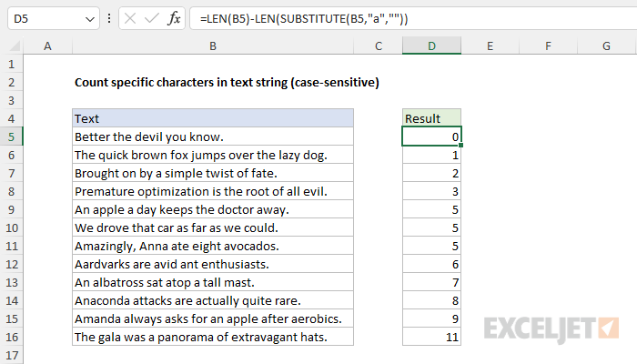
The LEN and SUBSTITUTE functions can be combined to count a specific character in a text string. The idea is to calculate the length of the original text string, then subtract the length of the text string after removing all occurrences of the character. In the example shown, the formula in cell D5 is:

=LEN(B5)-LEN(SUBSTITUTE(B5,"a",""))

This formula counts the number of a's that appear in cell B5. Notice the LEN function is used twice. The first LEN calculates the length of the original text string. The second LEN calculates the length of the text after all a's have been removed with the SUBSTITUTE function. Next, the result from the second LEN is subtracted from the result from the first LEN. The final result is the number of a's removed by SUBSTITUTE, which is equal to the count of a's in the original text. For example, with the text "banana" in cell A1, the formula calculates like this:

=LEN(A1)-LEN(SUBSTITUTE(A1,"a",""))
=LEN("banana")-LEN(SUBSTITUTE("banana","a",""))
=LEN("banana")-LEN("bnn")
=6-3
=3

Note that this formula is case-sensitive by default because the SUBSTITUTE function is case-sensitive. This means an uppercase "A" will not be counted. See below for an option that is not case-sensitive.

Case-insensitive option

SUBSTITUTE is a case-sensitive function, so it will match the case when replacing text. This means that the original formula above will not count the "A" in cell B9, because SUBSTITUTE is configured to look for lowercase "a". If you need a case-insensitive count, one solution is to add the LOWER function to the formula like this:

=LEN(B5)-LEN(SUBSTITUTE(LOWER(B5),"a",""))

In this formula, the LOWER function runs first to convert all text to lowercase. The result is returned to SUBSTITUTE and the formula then runs as before. All uppercase A's in the text are now lowercase, so they will be included in the count. The screen below shows the result:

Notice that the count is now higher in cases where the text in column B includes an uppercase "A" that was previously not counted.

Note: although we use the LOWER function in the above formula, an alternative approach is to use the UPPER function, and then search for an uppercase "A". Both options will return the same result.