Summary
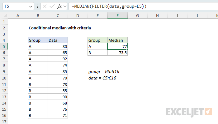
To calculate a conditional median based on one or more criteria, you can use the MEDIAN function together with the FILTER function. In the example shown, the formula in F5 is:
=MEDIAN(FILTER(data,group=E5))
where group (B5:B16) and data (C5:C16) are named ranges. FILTER returns only the values that match the criteria, then MEDIAN returns the median of those values. The result for group A is 77. There is also an older approach based on MEDIAN and IF that works in any version of Excel. Both are explained below.
Generic formula
=MEDIAN(FILTER(range,criteria))
Explanation
The MEDIAN function has no built-in way to apply criteria. Given a range of numbers, it simply returns the median, the middle value. And, unlike the SUMIFS, COUNTIFS, and AVERAGEIFS functions, there is no "MEDIANIFS" function. To calculate a median based on one or more conditions, we need to construct a formula that will feed MEDIAN only the values that meet criteria.
This page explains two formulas that do this: a modern approach based on the FILTER function, and an older approach with IF. Both return the same result, and each has tradeoffs worth understanding.
Table of contents
- What is a median?
- MEDIAN with FILTER
- MEDIAN with IF
- Error handling
- More than one condition
- Other functions
- Final thoughts
What is a median?
The median is the middle value in a set of numbers sorted from smallest to largest: half the values fall below the median and half fall above. When the set contains an odd number of values, the median is the single value in the middle. When the set contains an even number of values, the median is the average of the two middle values. This is different from the average (mean), which adds all the values and divides by the count, and from the mode, which is the value that appears most often.
In this example, group A contains six values: 80, 65, 92, 74, 85, and 70. Sorted, these become 65, 70, 74, 80, 85, 92. The two middle values are 74 and 80, so the median is 77 (their average). Group B works the same way and returns 73.5. Because each group contains an even number of values, both medians fall between two numbers, which is why group B returns 73.5 and not a value from the list. A result like 73.5 is correct, not a rounding error.
MEDIAN with FILTER
In modern versions of Excel that support dynamic arrays, the cleanest way to apply criteria is with the FILTER function. In the worksheet shown below, the formula in F5 is:
=MEDIAN(FILTER(data,group=E5))
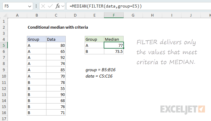
Working from the inside out, FILTER is configured to return values from data where group equals the value in E5 ("A"). The criteria compares each value in group to E5, which creates an array of TRUE and FALSE values:
{TRUE;TRUE;TRUE;TRUE;TRUE;TRUE;FALSE;FALSE;FALSE;FALSE;FALSE;FALSE}
FILTER uses this array to keep only the values from data that line up with TRUE and discards the rest. The result is an array of just the group A values:
{80;65;92;74;85;70}
This array is returned directly to MEDIAN, which returns the median, 77. Because FILTER gives MEDIAN only the matching values, the solution is clean and intuitive.
The named ranges group and data are used for convenience and readability only. The same formula works fine with ordinary range references:
=MEDIAN(FILTER(C5:C16,B5:B16=E5))
But note that if you want to copy the formula down from cell F5, you will want to use absolute references:
=MEDIAN(FILTER($C$5:$C$16,$B$5:$B$16=E5))
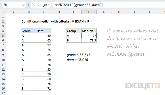
MEDIAN with IF
Another approach that pre-dates the FILTER function in Excel is to use MEDIAN with IF. This is the original approach to this problem, and it still works well. In the worksheet below, the formula in F5 looks like this:
=MEDIAN(IF(group=E5,data))
At the core, we are still filtering the data to include only values that meet criteria. However, instead of using the FILTER function, we are using the IF function. Inside MEDIAN, IF compares each value in group (B5:B16) to E5 and returns the matching value from data if the test is TRUE and FALSE if not, since no value is supplied for the false argument. The result is an array like this:
{80;65;92;74;85;70;FALSE;FALSE;FALSE;FALSE;FALSE;FALSE}
Notice that only the values associated with group A survive. Values associated with group B are converted to FALSE. This array is delivered directly to MEDIAN, which automatically ignores the FALSE values and returns the median of the remaining numbers, 77. The result is exactly the same as the FILTER formula.
In modern Excel (Microsoft 365 and Excel 2021+), this formula works normally with no special handling. In older versions (Excel 2019 and earlier), it is an array formula and must be entered with Control + Shift + Enter. If you open a workbook that already contains the formula in an older version, Excel will add the curly braces automatically, signifying an array formula:
{=MEDIAN(IF(group=E5,data))}
The formula will keep working without changes, but if the formula is edited, it must be re-entered with Control + Shift + Enter or otherwise it will fail. This has always been a subtle gotcha with old-style array formulas in Excel.
Error handling
One interesting difference between these two formula approaches is that they fail differently. If no rows match the criteria, MEDIAN with IF returns a #NUM! error, while MEDIAN with FILTER returns a #CALC! error.
The #CALC! error returned by FILTER is new in Excel with the introduction of dynamic array formulas, and many users won't know what to make of it when they see it. One option is to convert it to a more common #N/A error ("Not available") with the NA function like this:
=MEDIAN(FILTER(data,group=E5,NA()))
Another option you can use with both formulas is the IFERROR function which will trap and redirect any error in Excel:
=IFERROR(MEDIAN(FILTER(data,group=E5)),"No data")
=IFERROR(MEDIAN(IF(group=E5,data)),"No data")
Try it: Try the formulas above in the attached worksheets to see how they work.
Be aware that IFERROR is a blunt instrument that will suppress all errors, which can mask important information. For example, if you misspell a function name, Excel will return #NAME!, indicating an unrecognized function. But IFERROR will catch that error and return "No data" as configured above.
More than one condition
Both approaches can be extended to apply multiple criteria. With FILTER, use multiplication for AND logic, where all conditions must be true. For example, if you also had a region column:
=MEDIAN(FILTER(data,(group=E5)*(region=G5)))
Use addition for OR logic, where any condition can be true:
=MEDIAN(FILTER(data,(group="A")+(group="B")))
With MEDIAN and IF, you can nest a second IF:
=MEDIAN(IF(group=E5,IF(region=G5,data)))
or use Boolean logic to avoid the extra nesting:
=MEDIAN(IF((group=E5)*(region=G5),data))
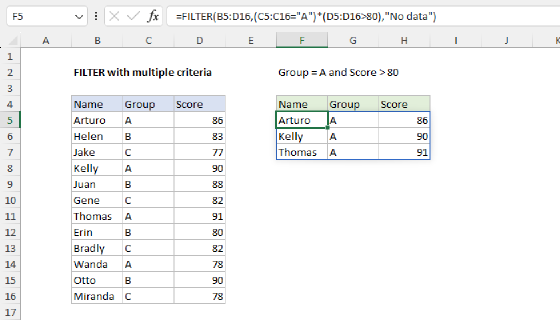
For more detail on building criteria with AND and OR logic, see Filter with multiple criteria.
Other functions
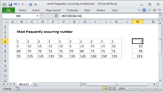
You can use both approaches above with other functions that don't handle conditions natively, such as the MODE and STDEV functions. Here are two examples with FILTER:
=MODE(FILTER(data,group=E5))
=STDEV(FILTER(data,group=E5))
In each case, FILTER narrows the data down to the rows that match your criteria, and the outer function does the rest.
Final thoughts
Both formulas work well to calculate a conditional median, but each approach has subtle tradeoffs:
- MEDIAN with IF is a bit shorter and arguably easier to read.
- MEDIAN with IF depends on MEDIAN ignoring FALSE values.
- FILTER is more modern and intuitive; a universal solution to filtering data.
- MEDIAN with IF works in every version of Excel.
- FILTER requires Excel 2021 or later.
Personally, I would use the FILTER approach unless I needed backward compatibility with an old version of Excel. Which formula do you prefer?