Biweekly pay schedule

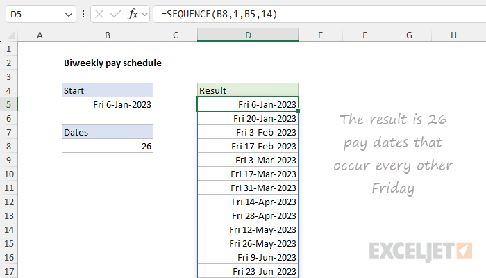
In this example, the goal is to create a list of pay dates that follow a biweekly schedule. A biweekly pay schedule means employees are paid every two weeks on a given day of the week. Each pay period is 14 days, and there are usually 26 pay dates per year, though occasionally 27 depending on the calendar. In the worksheet shown above, pay dates are every other Friday, beginning on the first Friday of the year. We can solve this problem with the SEQUENCE function, as explained below.

Background study

If you are unfamiliar with the SEQUENCE function, or dynamic array formulas in general, these links will help you get up to speed quickly:

• How to use the SEQUENCE function - overview
• The SEQUENCE function - 3 min video
• SEQUENCE of dates - 3 min video
• Dynamic Array Formulas - video training

SEQUENCE function

The SEQUENCE function is used to generate numeric sequences with the following syntax:

=SEQUENCE(rows,[columns],[start],[step])

• rows - the number of rows to return
• columns - the number of columns to return
• start - the starting value
• step - the increment to use between values

In this example, the goal is to generate a sequence of 26 pay dates, each 14 days apart. To generate the dates, the formula in cell D5 is:

=SEQUENCE(B8,1,B5,14)

Inside SEQUENCE, we provide the following values:

• rows - B8 (26)
• columns - 1
• start - B5 (January 6, 2023 = 44932)
• step - 14 (days between dates)

We can use SEQUENCE to generate dates in Excel because Excel dates are just large serial numbers. The serial number for January 1, 2023, is 44927, so the serial number for January 6, 2023, is 44932. The formula is evaluated by Excel's formula engine like this:

=SEQUENCE(B8,1,B5,14)
=SEQUENCE(26,1,44932,14)

Essentially, we are asking SEQUENCE for 26 numbers that start on 44927 and are incremented by 14. With the above configuration, SEQUENCE returns an array that contains 26 dates in serial number format:

{44932;44946;44960;44974;44988;45002;45016;45030;45044;45058;45072;45086;45100;45114;45128;45142;45156;45170;45184;45198;45212;45226;45240;45254;45268;45282}

These values spill into the range D5:D30. When properly formatted, they display as dates. In this particular example, we are using the custom number format below:

ddd d-mmm-yyyy

This causes Excel to display an abbreviated day name (i.e. "Fri") before the date to make it easy to verify correct results.

Holidays

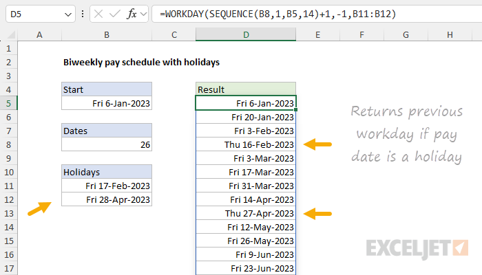
The formula above does not take into account pay dates that land on holidays, which are typically moved to the previous business day. One way to do this is to add in the WORKDAY function, which can calculate the next or previous workday from a given start date, taking into account weekends and holidays. The generic formula looks like this:

=WORKDAY(SEQUENCE(n,1,start,14)+1,-1,holidays)

Where n is the number of dates to generate, and holidays is a range or array that contains dates that are holidays. The worksheet below shows how this formula can be adapted to the worksheet discussed above:

Here, we basically feed the results from SEQUENCE directly into the WORKDAY function, with the range B11:B12 given for the holidays argument. We have to use a bit of trickery here to get WORKDAY to check the date returned by SEQUENCE. We do this by asking WORKDAY for the workday previous to the date + 1. In other words, we add 1 to the date, then ask WORKDAY for the previous workday by providing -1 for days. This causes WORKDAY to check the original date from SEQUENCE, and step back to the previous workday if the pay date is in fact a holiday. With the (arbitrary) dates of Feb 17, 2023, and April 28, 2023, provided as holidays in the range B11:B12, notice how the formula rolls back to Thursday in cells D8 and D13.