Summary
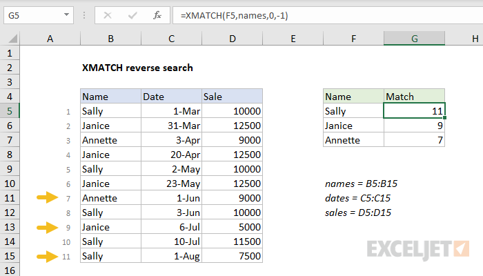
To perform a "reverse search" (i.e. search last to first), you can use the XMATCH function. In the example shown, the formula in cell G5, copied down, is:
=XMATCH(F5,names,0,-1)
where names (B5:B15) is a named range.
Generic formula
=XMATCH(A1,range,0,-1)
Explanation
The XMATCH function offers new features not available with the MATCH function. One of these is the ability to perform a "reverse search", by setting the optional search mode argument. The default value for search mode is 1, which specifies a normal "first to last" search. In this mode, XMATCH will match the lookup value against the lookup array, beginning at the first value.
=XMATCH(F5,names,0,1) // start with first name
Setting search mode to -1 species a "last to first" search. In this mode, XMATCH will match the lookup value against the lookup array, starting with the last value, and moving toward the first:
=XMATCH(F5,names,0,-1) // start with last name
Retrieve date and amount
XMATCH returns a position. Typically, XMATCH is used with the INDEX function to return a value at that position. In the example show, we can use INDEX and XMATCH together to retrieve the date and sales for each name as follows:
=INDEX(dates,XMATCH(F5,names,0,-1)) // get date
=INDEX(sales,XMATCH(F5,names,0,-1)) // get sale
where dates (C5:C15) and sales (D5:D15) are named ranges. As before, search mode is set to -1 to force a reverse search.
For more information about using INDEX with MATCH, see How to use INDEX and MATCH.
Dynamic Array Formulas are available in Office 365 only.