Summary
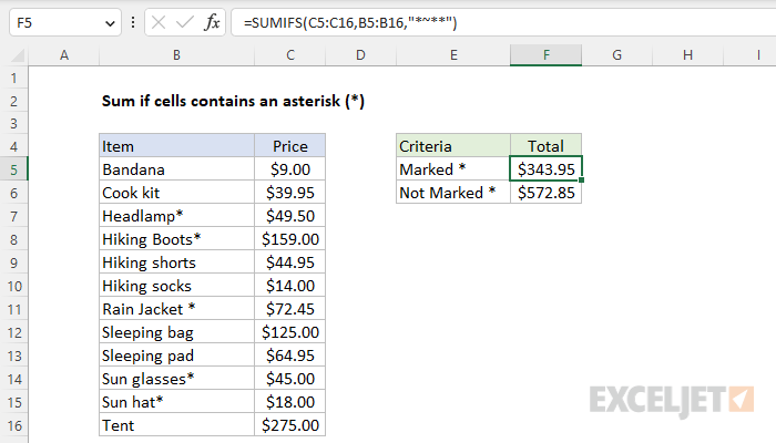
To sum numbers when corresponding cells contain an asterisk (*), you can use the SUMIFS function with criteria that uses the tilde (~) as an escape character. In the example shown, cell G6 contains this formula:
=SUMIFS(C5:C16,B5:B16,"*~**")
This formula sums the Price in column C when the Item name in column B contains an asterisk ("*").
Generic formula
=SUMIFS(sum_range,range,"*~**")
Explanation
The goal in this example is to sum Prices in column C when the Items in column B contain an asterisk (). The challenge is that the asterisk () is reserved as a wildcard in functions like the SUMIFS function, so you can't match a literal occurrence of this character without using a special syntax.
Wildcards
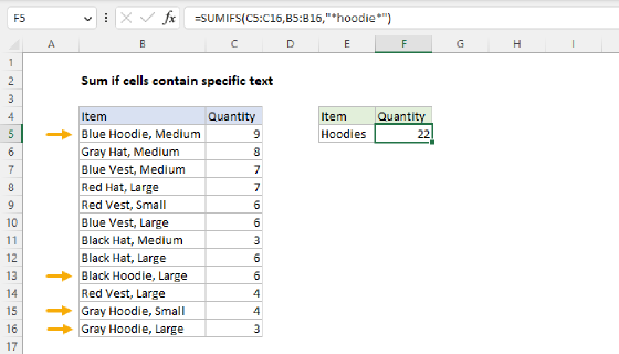
Excel functions like SUMIF and SUMIFS support the wildcard characters "?" (any one character) and "" (zero or more characters), which can be used in criteria. Wildcards allow you to create criteria to target cells that "begin with", "end with", "contain 3 characters" and so on. The table below shows some examples. For this problem, we want to use the "Cells that contain text in xyz" pattern, which uses two asterisks (), one before and one after the search string like this "xyz".
| Target | Criteria |
|---|---|
| Cells with 3 characters | "???" |
| Cells equal to "xyz", "xaz", "xbz", etc | "x?z" |
| Cells that begin with "xyz" | "xyz*" |
| Cells that end with "xyz" | "*xyz" |
| Cells that contain "xyz" | "xyz" |
| Cells that contain text in A1 | ""&A1&"" |
Because asterisks and question marks are themselves wildcards, if you want to search for these characters specifically, you'll need to escape them with a tilde (~). The tilde causes Excel to handle the next character literally.
SUMIFS solution
To sum Prices in column C when the Items in column B contain an asterisk (*), the formula in cell F5 is:
=SUMIFS(C5:C16,B5:B16,"*~**")
In this case we are using "~" to match a literal asterisk, but this is surrounded by asterisks on either side, in order to match an asterisk anywhere in the cell. If you just want to match an asterisk at the end of a cell, you can use "~" for the criteria. To sum Prices for Item names that do not contain an asterisk (""), the formula in cell F6 is:
=SUMIFS(C5:C16,B5:B16,"<>*~**")
This formula simply prepends the not equal to operator ("<>") to the existing criteria. For more details about using other operators in the SUMIFS function, see this page.
SUMIF solution
This problem can also be solved with the older SUMIF function, which only supports a single condition. The equivalent formulas based on SUMIF look like this:
=SUMIF(B5:B16,"*~**",C5:C16) // contains *
=SUMIF(B5:B16,"<>*~**",C5:C16) // does not contain *
Other options
In Excel, there is always another way to skin the cat. If you don't like the fiddly syntax needed to escape wildcards above, you can use a formula based on the FIND function to search for an asterisk directly. One option that will work in any version of Excel is SUMPRODUCT + FIND:
=SUMPRODUCT(ISNUMBER(FIND("*",B5:B16))*C5:C16)
This works because, unlike the SEARCH function, the FIND function does not support wildcards. Another option in newer versions of Excel is to use the SUM function with the FILTER function:
=SUM(FILTER(C5:C16,ISNUMBER(FIND("*",B5:B16)),0))
Note that both of these functions use the same logic to locate text that contains an asterisk: ISNUMBER + FIND. To read more about how this part of the formula works, see this example.