Summary
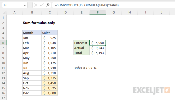
To sum values created by formulas only, you can use a formula based on the SUMPRODUCT and ISFORMULA functions. In the example shown, the formula in F6 is:
=SUMPRODUCT(ISFORMULA(sales)*sales)
where sales is the named range C5:C16. The result is $5950, the sum of the values in the range C13:C16, which are created with a formula.
Generic formula
=SUMPRODUCT(ISFORMULA(range)*range)
Explanation
In this example, the goal is to calculate a sum of the values in a range that are generated with a formula. In other words, we want to sum values in a range while ignoring the values that have been entered manually. In the context of this example, the hardcoded values in C5:C12 represent actual sales values and the values in the range C13:C16 represent forecasted values. This problem can be solved with a formula based on the SUMPRODUCT and ISFORMULA functions, as explained below.
Forecasted values
The forecasted values in the range C13:C16 are created with a formula based on the MROUND function. The formula in C13, copied down, is:
=MROUND(C12*1.05,25)
This formula is used to generate values that are 5% higher than the previous month, rounded to the nearest multiple of 25.
Sum formulas
To sum values in the range C5:C16 that are created with formulas, the formula in F6 is:
=SUMPRODUCT(ISFORMULA(sales)*sales)
This formula uses boolean logic to "filter" the numbers in sales (C5:C16) based on whether the values come from a formula or not. The ISFORMULA function created the filter like this:
ISFORMULA(sales)
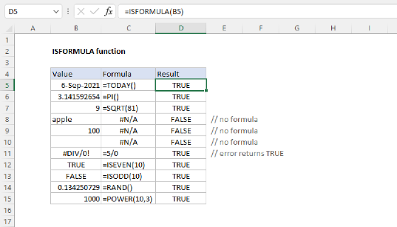
ISFORMULA returns TRUE when cell contains a formula, and FALSE if not. In this case, there are 12 values in the range C5:C16, so ISFORMULA returns 12 results in an array like this:
{FALSE;FALSE;FALSE;FALSE;FALSE;FALSE;FALSE;FALSE;TRUE;TRUE;TRUE;TRUE}
Each TRUE value in this array represents a cell that contains a formula. Notice the last 4 values are TRUE. When this array is multiplied by the named range sales (C5:C16), the math operation coerces the TRUE and FALSE values to 1s and 0s. We can visualize the formula at this point like this:
=SUMPRODUCT({0;0;0;0;0;0;0;0;1;1;1;1}*sales)
After the multiplication takes place, we have a single array like this:
=SUMPRODUCT({0;0;0;0;0;0;0;0;1375;1450;1525;1600})
Now you can see how the filter works. The values not created by formulas are "zeroed out". With just one array to process, SUMPRODUCT sums the array and returns a final result of 5950.
Not formulas
To sum values not generated by a formula, you can add the NOT function like this:
=SUMPRODUCT(NOT(ISFORMULA(sales))*sales)
This is the formula in cell F7. Here, the NOT function reverses the TRUE FALSE results returned by ISFORMULA function:
=SUMPRODUCT({1;1;1;1;1;1;1;1;0;0;0;0}*sales)
This causes the formula-created values to be zeroed out:
=SUMPRODUCT({925;1038;1105;1210;1250;1175;1230;1310;0;0;0;0})
The final result from this formula is 9243.