Sort by custom list

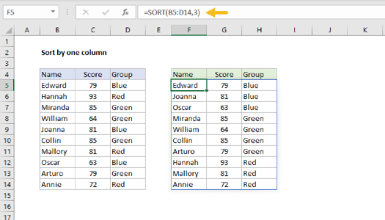
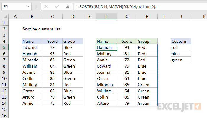
To sort a list in a custom order, you can combine the SORTBY function with the MATCH function. In the example shown, The table is being sorted by the "group" column using in the order shown in cells J5:J7. The formula in D5 is:

=SORTBY(B5:D14,MATCH(D5:D14,custom,0))

where custom is the named range J5:J7 that defines desired sort order.

Explanation

In this example, we are sorting a table with 10 rows and 3 columns. In the range J5:J7 (the named range custom), the colors "red", "blue", and "green" are listed in the desired sort order. The goal is to sort the table using values in the Group column in this same custom order.

The SORTBY function allows sorting based on one or more "sort by" arrays, as long as dimensions are compatible with the source data. In this case, we can't use the named range custom directly in SORTBY, because it only contains 3 rows while the table contains 10 rows.

However, to create an array with 10 rows that can be used as a "sort by" array, we can use the MATCH function like this:

MATCH(D5:D14,custom,0)

Notice we are passing in the Group values in D5:D14 as lookup values, and using custom as the lookup table. The result is an array like this:

{2;1;3;3;2;3;1;2;3;1}

Each value in the array represents the numeric position of given group value in custom, so there are 10 rows represented. This array is passed into the SORTBY function as the by_array1 argument. SORTBY sorts the table in the "red", "blue", "green" order and returns the result as a spill range starting in cell D5.