Summary
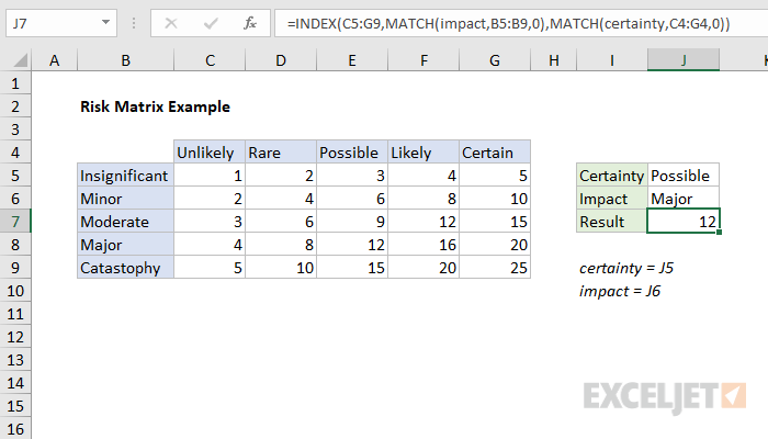
To set up a simple risk matrix, you can use a formula based on INDEX and MATCH. In the example shown, the formula in J7 is:
=INDEX(C5:G9,MATCH(impact,B5:B9,0),MATCH(certainty,C4:G4,0))
Where "impact" is the named range J6, and "certainty" is the named range J5
Context
A risk matrix is used for risk assessment. One axis is used to assign the probability of a particular risk and the other axis is used to assign consequence or severity. A risk matrix can a useful to rank the potential impact of a particular event, decision, or risk.
In the example shown, the values inside the matrix are the result of multiplying certainty by impact, on a 5-point scale. This is a purely arbitrary calculation to give each cell in the table a unique value.
Generic formula
=INDEX(matrix,MATCH(impact,range1,0),MATCH(certainty,range2,0))
Explanation
At the core, we are using the INDEX function to retrieve the value at a given row or column number like this:
=INDEX(C5:G9,row,column)
The range C5:C9 defines the matrix values. What's left is to figure out the correct row and column numbers, and for that we use the MATCH function. To get a row number for INDEX (the impact), we use:
MATCH(impact,B5:B9,0)
To get a column number for INDEX (the impact), we use:
MATCH(certainty,C4:G4,0)
In both cases, MATCH is set up to perform an exact match. When certainty is "possible" and impact is "major" MATCH calculates row and column numbers as follows:
=INDEX(C5:G9,4,3)
The INDEX function then returns the value at the fourth row and third column, 12.
For a more detailed explanation of how to use INDEX and MATCH, see this article.