Maximum value

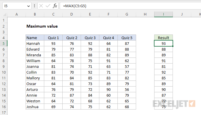
In this example, the goal is to get the maximum quiz score (i.e. the best quiz score) for each person listed in column B from the five quiz scores that appear in columns C through G. This is a job for the MAX function or the LARGE function, as explained below.

MAX function

The MAX function accepts one or more arguments, which can be a mix of constants, cell references, and ranges. MAX will return the maximum value in the data provided. Text values and empty cells are ignored.

In this example, each student has five test scores in the same row, and the goal is to get the maximum score for each student. Because the quiz scores are all together, the data is supplied to MAX as a single range. The formula in I5 is:

=MAX(C5:G5)

As the formula is copied down the table, MAX returns the highest score for each student. MAX is fully automatic. If data changes, MAX will automatically recalculate. Note that the MAX function will automatically ignore empty cells, but it will return an error if the data contains an error. To calculate a maximum value while ignoring errors, see this example.

LARGE function

The LARGE function can also be used to return the maximum value in a set of data. The generic syntax for LARGE looks like this:

=LARGE(range,n)

where n is a number like 1, 2, 3, etc. For example, you can retrieve the first, second, and third largest values like this:

=LARGE(range,1) // first largest
=LARGE(range,2) // second largest
=LARGE(range,3) // third largest

In this example, you could use LARGE to get the best quiz score for each person like this:

=LARGE(C5:G5,1)

The LARGE function is especially useful when you want to get other nth largest values, as seen in this example.

Notes

• To get a max value with one or more criteria, see the MAXIFS function. You can also use the FILTER function with the MAX function, as explained here.
• To get the nth largest value in a set of data (i.e. 1st largest, 2nd largest, 3rd largest, etc.), see the LARGE function.