Summary
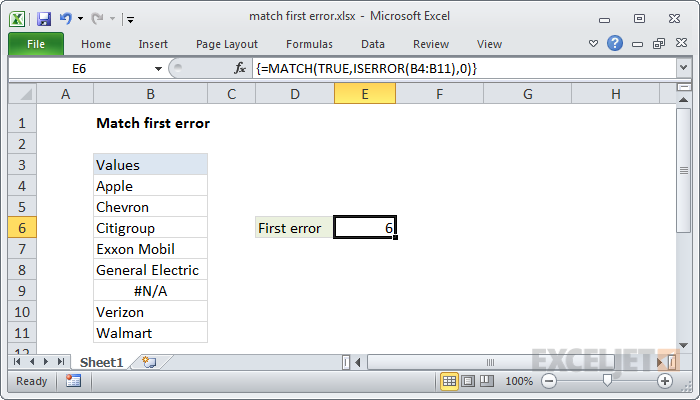
If you need to match the first error in a range of cells, you can use an array formula based on the MATCH and ISERROR functions. In the example shown, the formula is:
{=MATCH(TRUE,ISERROR(B4:B11),0)}
This is an array formula, and must be entered using Control + Shift + Enter (CSE).
Generic formula
{=MATCH(TRUE,ISERROR(rng),0)}
Explanation
Working from the inside out, the ISERROR function returns TRUE when a value is a recognized error, and FALSE if not.
When given a range of cells (an array of cells) ISERROR function will return an array of TRUE/FALSE results. In the example, this resulting array looks like this:
{FALSE;FALSE;FALSE;FALSE;FALSE;TRUE;FALSE;FALSE}
Note that the 6th value (which corresponds to the 6th cell in the range) is TRUE, since cell B9 contains #N/A.
The MATCH function is configured to match TRUE in exact match mode. It finds the first TRUE in the array created by ISERROR and returns the position. If no match is found, the MATCH function itself returns #N/A.
Finding the first NA error
The formula above will match any error. If you want to match the first #N/A error, just substitute ISNA for ISERROR:
{=MATCH(TRUE,ISNA(B4:B11),0)}