Summary
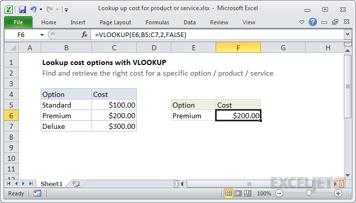
If you have a list of products or services (or related options), with associated costs, you can use VLOOKUP to find and retrieve the cost for a specific option.
In the example shown, the formula in cell F6 is:
=VLOOKUP(E6,B5:C7,2,FALSE)
This formula uses the value of cell E6 to lookup and retrieve the right cost in the range B5:C7.
Generic formula
=VLOOKUP(product,table,column,FALSE)
Explanation
This is a basic example of VLOOKUP in "exact match" mode. The lookup value is B6, the table is the range B5:C7, the column is 2, and the last argument, FALSE, forces VLOOKUP to do an exact match. (Read why this is necessary here).
If VLOOKUP finds a matching value, the associated cost will be retrieved from the 2nd column (column C). If no match is found, VLOOKUP will return the #N/A error.