Summary
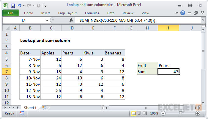
To lookup and return the sum of a column, you can use the a formula based on the INDEX, MATCH and SUM functions. In the example shown, the formula in I7 is:
=SUM(INDEX(C5:F11,0,MATCH(I6,C4:F4,0)))
Generic formula
=SUM(INDEX(data,0,MATCH(val,header,0)))
Explanation
The core of this formula uses the INDEX and MATCH function in a special way to return a full column instead of a single value. Working from the inside out, the MATCH function is used to find the correct column number for the fruit in I6:
MATCH(I6,C4:F4,0)
MATCH return 2 inside the INDEX function as the column_num argument, where the array is set to the range C5:F11, which includes data for all fruits.
The tricky part of the formula is the row_num argument, which is set to zero. Setting row to zero causes INDEX to return all values in the matching column in an array like this:
=SUM({6;12;4;10;0;9;6})
The SUM function then returns the sum of all items in the array, 47.