Summary
The #DIV/0! error appears when a formula attempts to divide by zero or a value equivalent to zero. Although a #DIV/0! error is caused by an attempt to divide by zero, it may also appear in other formulas that reference cells that display the #DIV/0! error. In the example shown, if any cell in A1:A5 contains a #DIV/0! error, the SUM formula below will also display #DIV/0!:
=SUM(A1:A5)
Generic formula
=IF(A2="","",A1/A2)
Explanation
About the #DIV/0! error
The #DIV/0! error appears when a formula attempts to divide by zero, or a value equivalent to zero. Like other errors, the #DIV/0! is useful, because it tells you there is something missing or unexpected in a spreadsheet. You may see #DIV/0! errors when data is being entered, but is not yet complete. For example, a cell in the worksheet is blank because data is not yet available.
Although a #DIV/0! error is caused by an attempt to divide by zero, it may also appear in other formulas that reference cells that display the #DIV/0! error. For example, if any cell in A1:A5 contains a #DIV/0! error, the SUM formula below will display #DIV/0!:
=SUM(A1:A5)
The best way to prevent #DIV/0! errors is to make sure data is complete. If you see an unexpected #DIV/0! error, check the following:
- All cells used by a formula contain valid information
- There are no blank cells used to divide other values
- The cells referenced by a formula do not already display a #DIV/0! error
Note: if you try to divide a number by a text value, you will see a #VALUE error not #DIV/0!.
#DIV/0! error and blank cells
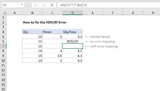
Blank cells are a common cause of #DIV/0! errors. For example, in the screen below, we are calculating quantity per hour in column D with this formula, copied down:
=B3/C3
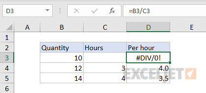
Because C3 is blank, Excel evaluates the value of C3 as zero, and the formula returns #DIV/0!.
#DIV/0! with average functions
Excel has three functions for calculating averages: AVERAGE, AVERAGEIF, and AVERAGEIFS. All three functions can return a #DIV/0! error when the count of "matching" values is zero. This is because the general formula for calculating averages is =sum/count, and count can sometimes be zero.
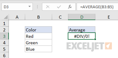
For example, if you try to average a range of cells containing only text values, the AVERAGE function will return #DIV/0! because the count of numeric values to average is zero:
Similarly, if you use the AVERAGEIF or AVERAGEIFS function with logical criteria that do not match any data, these functions will return #DIV/0! because the count of matching records is zero. For example, in the screen below, we are using the AVERAGEIFS function to calculate an average quantity for each color with this formula:
=AVERAGEIFS(quantity,color,E3)
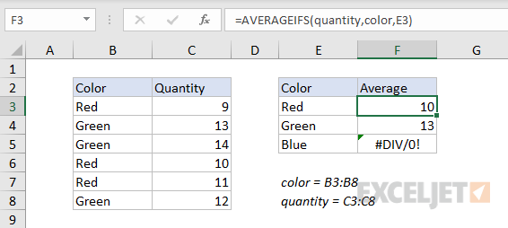
where "color" (B3:B8) and "quantity" (C3:C8) are named ranges.
Because there is no color "blue" in the data (i.e. the count of "blue" records is zero), AVERAGEIFS returns #DIV/0!.
This can be confusing when you are "certain" there are matching records. The best way to troubleshoot is to set up a small sample of hand-entered data to validate the criteria you are using. If you are applying multiple criteria with AVERAGEIFS, work step by step and only add one criteria at a time.
Once you get the example working with criteria as expected, move to real data. More information on formula criteria here.
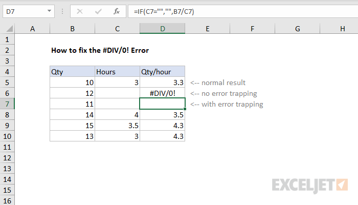
Trapping the #DIV/0! error with IF
A simple way to trap the #DIV/0! is to check required values with the IF function. In the example shown, the #DIV/0! error appears in cell D6 because cell C6 is blank:
=B6/C6 // #DIV/0! because C6 is blank
To check that C6 has a value and abort the calculation if no value is available, you can use IF like this:
=IF(C6="","",B6/C6) // display nothing if C6 is blank
You can extend this idea further and check that both B6 and C6 have values using the OR function:
=IF(OR(B6="",C6=""),"",B6/C6)
See also: IF cell is this OR that.
Trapping the #DIV/0! error with IFERROR
Another option for trapping the #DIV/0! error is the IFERROR function. IFERROR will catch any error and return an alternative result. To trap the #DIV/0! error, wrap the IFERROR function around the formula in D6 like this:
=IFERROR(B6/C6,"") // displays nothing when C6 is empty
Add a message
If you want to display a message when you trap a #DIV/0! error, just wrap the message in quotes. For example, to display the message "Please enter hours", you can use:
=IFERROR(B6/C6,"Please enter hours")
This message will be displayed instead of #DIV/0! while C6 remains blank.