Explanation
This formula takes advantage of the fact that TRIM will remove any number of leading spaces. We look for line breaks and "flood" the text with spaces where we find one. Then we come back and grab text from the right.
Working from the inside out, we use the SUBSTITUTE function to find all line breaks (char 10) in the text, and replace each one with 200 spaces:
SUBSTITUTE(B5,CHAR(10),REPT(" ",200))
After the substitution, the looks like this (with hyphens marking spaces for readability):
line one----------line two----------line three
With 200 spaces between each line of text.
Next, the RIGHT function extracts 200 characters, starting from the right. The result will look like this:
-------line three
Finally, the TRIM function removes all leading spaces, and returns the last line.
Note: 200 is an arbitrary number that represents the longest line you expect to find in a cell. If you have longer lines, increase this number as needed.
Mac version
Mac Excel uses a different line break character inside cells, char 13, so use this version of the formula instead:
=TRIM(RIGHT(SUBSTITUTE(B5,CHAR(13),REPT(" ",200)),200))
In Excel 365, both Win and Mac versions of Excel use CHAR(10) as a line break.


