Summary
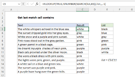
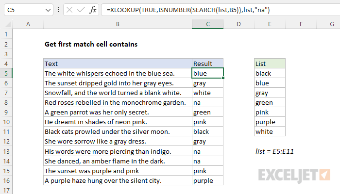
This article provides a method to search through a cell for one of several specified values, returning the first match found. The method uses the XLOOKUP function and the formula that appears in cell C5 of the worksheet is:
=XLOOKUP(TRUE,ISNUMBER(SEARCH(list,B5)),list,"na")
where list is the named range E5:E11. As the formula is copied down, it returns the first match found in each cell. If no match is found, it returns "na". The value to return if no match is found can be customized as desired.
Note: It is also possible to list all matches a cell contains with a formula.
Generic formula
=XLOOKUP(TRUE,ISNUMBER(SEARCH(list,A1)),list)
Explanation
The general goal is to search through a cell for one of several specified values and return the first match found if one exists. The worksheet includes a list of colors in the range E5:E11 (which is named list) and a series of short sentences in the range B5:B16. The task is to add a formula in column C that will search through each sentence in B5:B16 and extract the first color in E5:E11 that is found in each sentence. If no matching colors are found, the formula should return the value "na". One way to solve this problem is with a formula that utilizes the ISNUMBER, SEARCH, and XLOOKUP functions. In older versions of Excel, you can use a formula based on INDEX and MATCH. Both methods are explained below.
The functions
Let's first run through the functions used in the XLOOKUP formula:
- The ISNUMBER function checks if the given input or expression results in a number. It returns TRUE if the value is numeric, and FALSE if not.
- The SEARCH function is used to find the starting position of a specific substring within a string. The syntax is SEARCH(find_text, within_text, [start_num]). If the substring (find_text) is found, SEARCH returns the starting position as a number. If not, it results in an error.
- The XLOOKUP function is a modern upgrade to the older VLOOKUP function. XLOOKUP allows you to search for a key value in a specified range or array, and return a corresponding value from another range or array. The syntax is XLOOKUP(lookup_value, lookup_array, return_array, [if_not_found], [match_mode], [search_mode]).
The formula
Now, let's look at the formula that appears in cell C5:
=XLOOKUP(TRUE,ISNUMBER(SEARCH(list,B5)),list,"na")
Here's how the formula works step by step, working from the inside out:
SEARCH(list,B5)
The SEARCH function tries to find each color in the named range list (E5:E11) inside the sentence in cell B5. If a color is found, SEARCH returns the starting position as a number. If a color is not found, SEARCH returns an error. Because E5:E11 contains 7 colors, SEARCH returns 7 results in an array like this:
{#VALUE!;30;#VALUE!;#VALUE!;#VALUE!;#VALUE!;5}
Notice the second value is 30 and the seventh value is 5. These numbers indicate the numeric positions of the colors "white" and "blue" in cell B5. The #VALUE! errors indicate colors in E5:E11 that were not found. We need to convert these values into something more useful and for that, we use the ISNUMBER function:
ISNUMBER(SEARCH(list,B5))
This function is an error handler. Since the SEARCH function will return an error if the color is not found, ISNUMBER is used to turn the errors into FALSE (not a number) and the numbers (which indicate positions) into TRUE (is a number). The result from ISNUMBER is an array like this:
{FALSE;TRUE;FALSE;FALSE;FALSE;FALSE;TRUE}
Note we have TRUE in the second and seventh positions, indicating a match on the colors White and Blue. Next, we have the XLOOKUP function, which is the main part of the formula
=XLOOKUP(TRUE,ISNUMBER(SEARCH(list,B5)),list,"na")
After ISNUMBER and SEARCH are evaluated, the array from ISNUMBER is returned to XLOOKUP as the lookup_array argument:
=XLOOKUP(TRUE,{FALSE;TRUE;FALSE;FALSE;FALSE;FALSE;TRUE},list,"na")
XLOOKUP is configured to match the first TRUE in the array. When it finds a TRUE, it returns the corresponding color from the named range list (E5:E11). If no TRUE is found (i.e., no color from the list was found in the sentence), it returns "na". This value can be omitted or customized as desired. To recap, this formula extracts the first color found from the list (E5:E11) in each cell from B5 to B16. It does so by searching for each color in the sentence, checking whether the result is a number (indicating a match was found), and then returning the corresponding color.
First match in sentence, or first match in list?
The language used in this example is ambiguous because it is not clear whether we are referring to the "first color found in the list of colors" or the "first color found in each sentence". These are two distinctly different operations. The formula above returns the first match found in the color list. If multiple colors from the list appear in a sentence, the formula will return the color that appears first in the color list, not the color that occurs first in the sentence. If instead, you want to find the first matched color in a sentence (ignoring the order of colors in the list) we need to use a different formula like this:
=XLOOKUP(1,IFERROR(SEARCH(list,B5),0),list,"na",1)
This version of the formula has the same basic structure as the original formula. However, instead of using the ISNUMBER function as an error handler, it uses the IFERROR function. IFERROR is set to catch errors from SEARCH and remap them to a zero (0) value. After IFERROR runs, the lookup_array inside XLOOKUP looks like this:
=XLOOKUP(1,{0;34;0;0;0;0;5},list,"na",1)
XLOOKUP is configured to look for 1, and match_mode is set to 1, which means "exact match or next larger value". In this case, XLOOKUP will match the last value (5), because it is the next larger value after 1, and return "white", since "white" appears before "blue" in the sentence.
For more details on XLOOKUP, see How to use the XLOOKUP function.
INDEX and MATCH
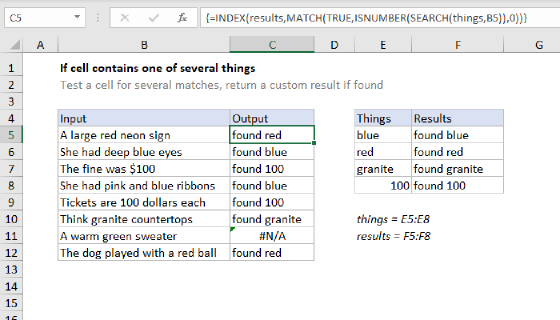
In older versions of Excel that do not provide XLOOKUP, you can solve this problem with a formula based on INDEX and MATCH:
=INDEX(list,MATCH(TRUE,ISNUMBER(SEARCH(list,B5)),0))
Note: this is an array formula and must be entered with control + shift + enter in Excel 2019 and older.
This formula works in much the same way as the XLOOKUP version above. Working from the inside out, we use ISNUMBER and SEARCH to locate color matches in each sentence like this:
ISNUMBER(SEARCH(list,B5)
As explained above, SEARCH will return the positions of any colors that appear in each sentence, and ISNUMBER will convert results from SEARCH into TRUE and FALSE values. The result is delivered to the MATCH function as the lookup_array:
=INDEX(list,MATCH(TRUE,{FALSE;TRUE;FALSE;FALSE;FALSE;FALSE;TRUE},0))
Notice MATCH is configured to look for TRUE, and there are 2 TRUE values in the lookup_array. The match_type argument is set to zero (0) to force an exact match. In this configuration, MATCH will match the first TRUE value and return 2 as a result directly to INDEX as the row_num argument:
=INDEX(list,2) // returns "blue"
INDEX will then return the second color in E5:E11 ("blue") as a final result.
First match in sentence
As above, we need a different INDEX and MATCH formula to extract the first color that appears in a sentence, as opposed to the first color matched in list (E5:E11):
=INDEX(list,MATCH(AGGREGATE(15,6,SEARCH(list,B5),1),SEARCH(list,B5),0))
The main trick in this formula is the lookup_value inside the MATCH function, which is calculated with the AGGREGATE function like this:
AGGREGATE(15,6,SEARCH(list,B5),1) // get min value
Here, we use AGGREGATE to get the minimum value in the results returned by SEARCH. We need AGGREGATE because the array will contain errors (returned by SEARCH when colors aren't found), and we need a function that will ignore those errors and still give us the minimum numeric value. AGGREGATE works well here because it has an option to ignore errors. The result from AGGREGATE is 5, which is returned to MATCH as the lookup_value. The lookup_array is created by the SEARCH function:
{#VALUE!;34;#VALUE!;#VALUE!;#VALUE!;#VALUE!;5}
We don't use ISNUMBER in this case because we need to be able to find the number calculated by AGGREGATE. Back in the formula, we now have:
=INDEX(list,MATCH(5,{#VALUE!;34;#VALUE!;#VALUE!;#VALUE!;#VALUE!;5},0))
The result from MATCH is 7, because 5 is the seventh value in the lookup_array. MATCH returns this number to INDEX as the row_num argument:
=INDEX(list,7) // returns "white"
The final result is "white", the first color found in the sentence.
For more details on INDEX with MATCH, see How to use the INDEX and MATCH.