Get column name from index in table

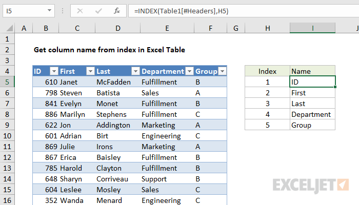
To get the name of a column in an Excel Table from its numeric index, you can use the INDEX function with a structured reference. In the example shown, the formula in I4 is:

=INDEX(Table1[#Headers],H5)

When the formula is copied down, it returns an name for each column, based on index values in column H.

Explanation

This is a standard INDEX formula. The only trick to the formula is the use of a structured reference to return a range for the table headers:

Table1[#Headers]

This range goes into INDEX for the array argument, with the index value supplied from column H:

=INDEX(Table1[#Headers],H5)

The result is the name of the first item in the header, which is "ID".

Although the headers are in a horizontal array, with values in columns, INDEX will use the row number as a generic INDEX for one-dimensional arrays like this and correctly return the value at that position.