Summary
To find and replace multiple values (i.e., perform a batch replace all operation), you can use the REDUCE function with a custom LAMBDA function to perform multiple substitutions in a single operation. In the example shown, the formula in D5 is:
=LET(
    range,B5:B16,
    find,F5:F9,
    replace,G5:G9,
    ix,SEQUENCE(ROWS(find)),
    result,REDUCE(range,ix,LAMBDA(a,i,
        SUBSTITUTE(a,INDEX(find,i),INDEX(replace,i))
    )),
    TRIM(result)
)
This is a tricky formula! In a nutshell, it runs through the values in B5:B16 one at a time. Then, for each value, it loops over the five find/replace pairs in G5:G9 and performs a "replace all" with each. The final modified values in column D are returned with a single formula. See the article below for a full teardown. I also explain how to adapt the formula to use regex and how to define it as a custom function you can call like a regular Excel function.
This formula is automatically case-sensitive because SUBSTITUTE is case-sensitive. If you need more functionality, you can optionally replace the SUBSTITUTE function with the REGEXREPLACE function as explained below.
Explanation
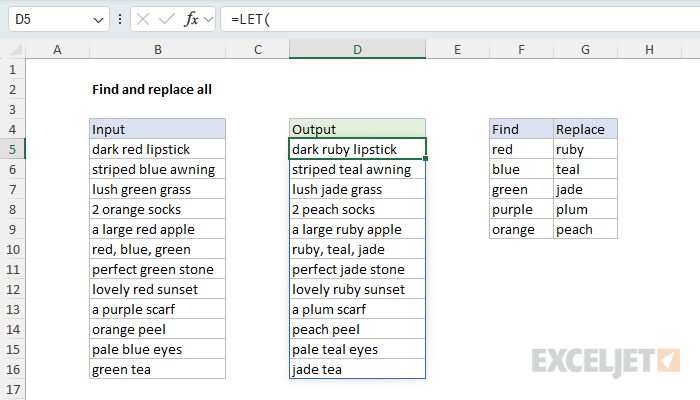
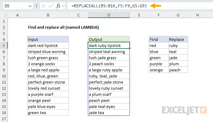
There is no built-in function to perform a series of find and replace operations in Excel, but you can create a formula that does the same thing. The goal in this example is to replace multiple ("find") values with corresponding ("replace") values in a single "replace all" operation. The text strings to process are in column B. The "find" and "replace" values appear in the table shown in columns F and G. For each text string in column B, we want to find and replace each value in column F with the corresponding value in column G. For example, every instance of "red" should be replaced with "ruby", every instance of "blue" should be replaced with "teal", and so on. The final output in column D is generated with a single formula like this in cell D5:
=LET(
    range,B5:B16,
    find,F5:F9,
    replace,G5:G9,
    ix, SEQUENCE(ROWS(find)),
    result, REDUCE(range,ix,LAMBDA(a,i,
        SUBSTITUTE(a,INDEX(find,i), INDEX(replace,i))
    )),
    TRIM(result)
)
The formula shown above features the REDUCE function, one of Excel's newer dynamic array functions. If you are using an older version of Excel that doesn't include the REDUCE function, it is possible to achieve the same result by nesting multiple SUBSTITUTE functions together in a more complicated formula, as explained below.
Table of contents
- Naming variables with the LET function
- Creating an array of indices
- Using REDUCE with lifting
- Inside the LAMBDA function
- Cleaning up the result
- More substitutions and dynamic ranges
- Using REGEXREPLACE for word boundaries
- Creating a custom function with a named LAMBDA
- Solution for Legacy Excel
Naming variables with the LET function
The formula uses the LET function to organize variables and make the formula easier to read and maintain. The first three variables define the input ranges:
=LET(
    range,B5:B16,
    find,F5:F9,
    replace,G5:G9,
The variable range contains the text strings to process, find contains the values to search for, and replace contains the corresponding replacement values. With these variables in place, we can refer to these ranges by name in the formula, which makes the logic easier to follow.
Creating an array of indices
Next, we use the SEQUENCE function to create a sequence of numbers that corresponds to the number of "find/replace" pairs, and assign the sequence to the variable ix:
ix,SEQUENCE(ROWS(find)),
Since there are 5 rows in the range F5:F9 (red, blue, green, purple, orange), the ROWS function returns 5, and SEQUENCE returns the array {1;2;3;4;5}. This array serves two purposes: (1) it gives us a list of indices that we can use with the INDEX function to retrieve corresponding "find" and "replace" values, and (2) it gives us an array that REDUCE can iterate over.
Using REDUCE with lifting
The core of the formula is the REDUCE function, which applies a series of substitutions to each text string:
result,REDUCE(range,ix,LAMBDA(a,i,
    SUBSTITUTE(a,INDEX(find,i),INDEX(replace,i))
)),
This is a clever use of REDUCE that takes advantage of a built-in process called "lifting". If you haven't seen this pattern before, it is somewhat tricky to understand. The key is to look at what is provided as the initial_value and what is provided as the array. Normally, we would expect the values to process (B5:B16) to be provided as the array argument. However, in this formula, the values to process are provided as the initial_value, and the array of indices ix from the previous step is provided as the array argument. In the dynamic array version of Excel, when you call a function that expects a single (scalar) value for an argument with an array of values, Excel "lifts" the function and calls it once for each value in the array, causing the function to return multiple results. This setup means we are actually calling the REDUCE function 12 times (once for each value in the range B5:B16). Then, for each value in B5:B16, REDUCE iterates over the array of indices and applies the custom LAMBDA function.
Inside the LAMBDA function
The actual search and replace operation is done inside the LAMBDA function, which looks like this:
LAMBDA(a,i,SUBSTITUTE(a,INDEX(find,i),INDEX(replace,i)))
The a argument is the accumulator, which holds the current value from the range B5:B16. The i argument is the current index from the array {1;2;3;4;5}. Inside the LAMBDA, the SUBSTITUTE function performs the actual replacement. The INDEX function retrieves the "find" value and the "replace" value using the current index i:
INDEX(find,i)    // gets the value to find
INDEX(replace,i) // gets the replacement value
For example, when i is 1, INDEX retrieves "red" from the find range and "ruby" from the replace range. SUBSTITUTE then replaces all instances of "red" with "ruby" in the current text string. The result from SUBSTITUTE becomes the new accumulator value, which is used as the starting point for the next iteration. This process continues for all indices (1 through 5), applying each substitution in sequence. When all substitutions have been completed for a given text string, REDUCE moves on to the next text string in the range B5:B16.
Cleaning up the result
The final step wraps the result from REDUCE in the TRIM function:
TRIM(result)
The TRIM function removes any extra spaces from the text strings. This is a safety measure that cleans up the output in case any of the substitutions create extra whitespace.
More substitutions and dynamic ranges
You can easily extend this formula to handle more find/replace pairs by adding more rows to the table in columns F and G. Then, update the ranges in the formula as needed to include the new rows. The rest of the formula will automatically adjust because it uses the ROWS function to determine how many pairs to process. If you want dynamic ranges that expand to include new find/replace rows automatically, you can use an Excel Table, the new TRIMRANGE function, or the related dot operator. For example, to make the formula dynamic up to the first 100 rows in the worksheet, you could use the dot operator when defining the first three variables like this:
=LET(
    range,B5:.B100,
    find,F5:.F100,
    replace,G5:.G100,
Note that 100 is just an arbitrary number to keep things simple; use a number that makes sense for your use case.
Using REGEXREPLACE for word boundaries
If you need better control over word boundaries (i.e., you don't want to match "red" inside "bored"), you can replace the SUBSTITUTE function with the REGEXREPLACE function like this:
=LET(
    range,B5:B16,
    find,F5:F9,
    replace,G5:G9,
    ix,SEQUENCE(ROWS(find)),
    result,REDUCE(range,ix,LAMBDA(a,i,
        REGEXREPLACE(a,"\b"&INDEX(find,i)&"\b",INDEX(replace,i))
    )),
    TRIM(result)
)
The \b is a regex word boundary marker that ensures matches only occur at word boundaries. You can also extend the call to REGEXREPLACE to include options for occurrence and case-sensitivity if needed. If you are new to Regular Expressions (regex) in Excel, see our regex guide here.
Creating a custom function with a named LAMBDA
To make it easier to use the formulas on this page, you can create a custom function via a "named LAMBDA". The first step is to wrap the function inside an outer LAMBDA, and list variable inputs as arguments. For example, to restructure the REGEXREPLACE version of the formula, you can create a formula like this:
=LAMBDA(range,find,replace,
    LET(
        ix, SEQUENCE(ROWS(find)),
        result, REDUCE(range, ix, LAMBDA(a,i,
            REGEXREPLACE(a, "\b"&INDEX(find, i)&"\b", INDEX(replace, i))
        )),
        TRIM(result)
    )
)
The second step is to name the LAMBDA using the Name Manager in Excel. For example, we could call this function REPLACEALL:
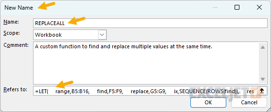
You can invoke the New Name window via Formulas > Name Manager > New (or use the keyboard shortcut Control + F3 to bring up the Name Manager, then click New). Once the name has been created, you can use it like a regular function in Excel:
You can name the function anything that makes sense to you, i.e., REPLACEALL, SUBSTITUTEALL, MULTIREPLACE, etc. The name will appear in the formula bar as shown.
You can extend the LAMBDA to an argument for case-sensitivity if needed. Just add a new argument called "case" or "case-sensitivity", and include that argument when REGEXREPLACE is called inside the formula. You will also need to include an extra comma for the optional occurrence argument before adding the case-sensitivity, which needs to be 0 (case-sensitive) or 1 (case-insensitive). The default is 0 for a case-sensitive match.
Solution for Legacy Excel
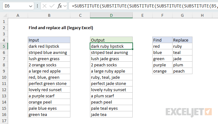
If you are using an older version of Excel that doesn't include the REDUCE function, you can achieve the same result by nesting multiple SUBSTITUTE functions together. However, this approach is less flexible and more difficult to maintain than the REDUCE-based solution above. With nested SUBSTITUTE functions, you need to manually add or remove function calls each time you change the number of find/replace pairs, and the formula quickly becomes difficult to read. The formula used in the worksheet below looks like this:
=SUBSTITUTE(SUBSTITUTE(SUBSTITUTE(SUBSTITUTE(SUBSTITUTE(B5,INDEX(find,1),INDEX(replace,1)),INDEX(find,2),INDEX(replace,2)),INDEX(find,3),INDEX(replace,3)),INDEX(find,4),INDEX(replace,4)),INDEX(find,5),INDEX(replace,5))
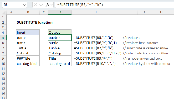
The formula uses the SUBSTITUTE function to perform each substitution, feeding in find/replace pairs from a table using the INDEX function. The basic pattern looks like this:
=SUBSTITUTE(text,find,replace)
where "text" is the incoming value, "find" is the text to look for, and "replace" is the text to replace with. To perform multiple substitutions, you nest SUBSTITUTE functions together, with each subsequent SUBSTITUTE beginning with the result from the previous SUBSTITUTE, where "find" is a named range containing the values to find (F5:F9), and "replace" is a named range containing the replacement values (G5:G9). The INDEX function retrieves both the "find" text and the "replace" text like this:
INDEX(find,1) // first "find" value
INDEX(replace,1) // first "replace" value
So, to run the first substitution (look for "red", and replace it with "pink"), we use:
=SUBSTITUTE(B5,INDEX(find,1),INDEX(replace,1))
The INDEX function makes this solution "dynamic" – if any of the values in the find/replace table are changed, results update immediately.
Line breaks for readability
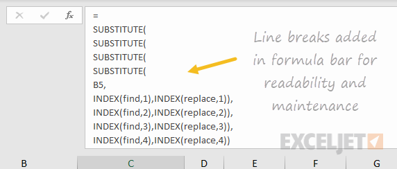
You'll notice this kind of nested formula is quite difficult to read. By adding line breaks, you can make the formula much easier to read and maintain:
=
SUBSTITUTE(
SUBSTITUTE(
SUBSTITUTE(
SUBSTITUTE(
SUBSTITUTE(
B5,
INDEX(find,1),INDEX(replace,1)),
INDEX(find,2),INDEX(replace,2)),
INDEX(find,3),INDEX(replace,3)),
INDEX(find,4),INDEX(replace,4)),
INDEX(find,5),INDEX(replace,5))
The formula bar in Excel ignores extra white space and line breaks, so the above formula can be pasted in directly.
To expand and collapse the formula bar quickly, use the keyboard shortcut Control + Shift + U
More substitutions
More rows can be added to the table to handle more find/replace pairs. Each time a pair is added, the formula needs to be updated to include the new pair. It's also important to make sure the named ranges (if you are using them) are updated to include new values as needed. Alternately, you could use a proper Excel Table to hold the find and replace values, instead of named ranges, then adjust the formula to refer to the table.
Other uses
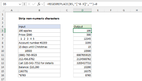
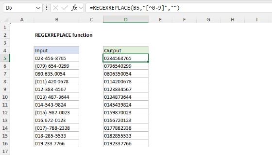
The same approach can be used to clean up text by "stripping" punctuation and other symbols from text with a series of substitutions. For example, the formula on this page shows how to clean and reformat telephone numbers.