Explanation
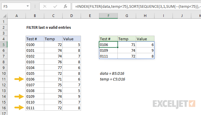
The goal in this example is to display the last 3 valid entries from the table shown, where "valid" is defined as a temperature of less than 75 in the "Temp" column. At a high level, the FILTER function is used to filter entries based on a logical test, and the INDEX function is used to extract the last 3 entries from the filtered list. Working from the inside out, we use the SEQUENCE function to construct a row number value for the INDEX function like this:
SORT(SEQUENCE(3,1,SUM(--(temp<75)),-1))
SEQUENCE is configured to create an array of 3 rows x 1 column. The step value is -1, and the start number is defined by this snippet:
SUM(--(temp<75)) // returns 7
Here we are counting temp values less than 75. Because the named range temp contains twelve values, the result is an array of 12 TRUE and FALSE values:
{TRUE;TRUE;TRUE;FALSE;FALSE;TRUE;TRUE;FALSE;FALSE;TRUE;FALSE;TRUE}
The double negative (--) is used to coerce the TRUE and FALSE results to 1s and 0s, and the SUM function returns the total:
SUM({1;1;1;0;0;1;1;0;0;1;0;1}) // returns 7
This number is returned directly to SEQUENCE for the start value. Now we have:
=SORT(SEQUENCE(3,1,7,-1))
=SORT({7;6;5})
={5;6;7}
We use SORT to ensure that values are returned in the same order they appear in the source data. This array is handed off to the INDEX function as the row_num argument:
=INDEX(FILTER(data,temp<75),{5;6;7},SEQUENCE(1,COLUMNS(data)))
In a similar way, SEQUENCE is also used to generate an array for columns:
SEQUENCE(1,COLUMNS(data)) // returns {1,2,3}
which is given to INDEX for the columns argument. Now we have:
=INDEX(FILTER(data,temp<75),{5;6;7},{1,2,3})
The next step is to construct the array for INDEX to work with. We only want to work with "valid" entries, so we use the FILTER function to retrieve a list of entries where the temp value is less than 75:
FILTER(data,temp<75)
The array argument is data, and the include argument is the expression temp<75. This can be translated literally as "return values from the named range data where values in temp are less than 75". The result is a 2D array with 3 columns and 7 rows:
{"0100",72,5;"0101",74,8;"0102",74,7;"0105",72,8;"0106",71,6;"0109",74,9;"0111",72,8}
Notice rows associated temp values greater than or equal to 75 have been removed. This array is returned to the INDEX function for its array argument.
Finally, the INDEX function returns the last 3 entries from the array returned by FILTER.
Note: Both the value for n and the logic used to test for valid entries is arbitrary in this example and can be adjusted as needed to suit your needs.


