Summary
To create a hyperlink from a lookup, you can use the VLOOKUP function together with the HYPERLINK function.
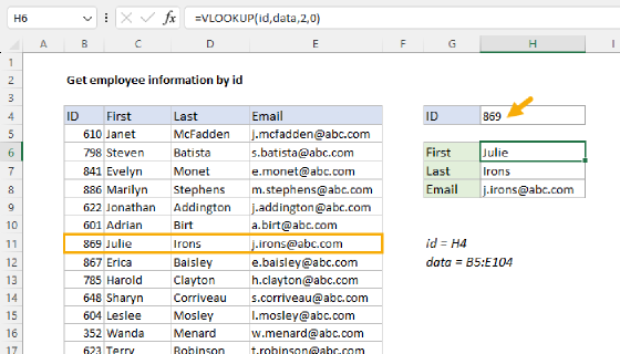
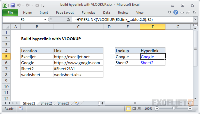
In the example shown, the formula in F5 is:
=HYPERLINK(VLOOKUP(E5,link_table,2,0),E5)
Generic formula
=HYPERLINK(VLOOKUP(name,table,column,0),name)
Explanation
The hyperlink function allows you to create a working link with a formula. It takes two arguments: link_location and, optionally, friendly_name.
Working from the inside out, VLOOKUP looks up and retrieves a link value from column 2 of the named range "link_table" (B5:C8). The lookup value comes from column E, and VLOOKUP is configured for exact match.
The result is fed into HYPERLINK as link_location, and the text in column E is used for friendly_name.
HYPERLINK returns a working link.