Summary
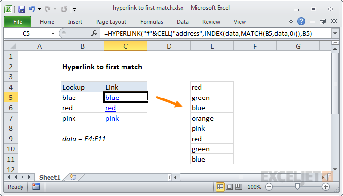
To create hyperlinks to the first match in a lookup, you can use a formula based on the HYPERLINK function, with help from CELL, INDEX and MATCH. In the example shown, the formula in C5 is:
=HYPERLINK("#"&CELL("address",INDEX(data,MATCH(B5,data,0))),B5)
This formula generates a working hyperlink to the first match found of the lookup value in the named range "data".
Generic formula
=HYPERLINK("#"&CELL("address",INDEX(data,MATCH(val,data,0))),val)
Explanation
Working from the inside out, we use a standard INDEX and MATCH function to locate the first match of lookup values in column B:
INDEX(data,MATCH(B5,data,0))
The MATCH function gets the position of the value in B5 inside the named range data, which for the lookup value "blue" is 3. This result goes into the INDEX function as row_num, with "data" as the array:
INDEX(data,3)
This appears to return the value "blue" but in fact the INDEX function returns the address E6. We extract this address using the CELL function, which is concatenated to the "#" character:
=HYPERLINK("#"&CELL(E6,B5)
In this end, this is what goes into the HYPERLINK function:
=HYPERLINK("#$E$6","blue")
The HYPERLINK function then constructs a clickable link to cell E6 on the same sheet, with "blue" as the link text.