Summary
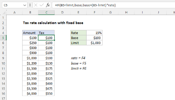
This example uses the VLOOKUP function to calculate a simple tax rate. In the example shown, the formula in C5 is:
=VLOOKUP(B5,tax_data,2,1)
where tax_data is the named range F5:G9. As the formula is copied down column C, the VLOOKUP function looks up the income in column B in the range F5:F9 and returns the correct tax rate from the range G5:G9. A formula in column D multiples the income by the tax rate to display the total tax amount.
Note: this formula calculates a tax rate in a simple one-tier scheme. To calculate tax based on a progressive system where income is taxed at different rates in multiple tiers, see this example.
Generic formula
=VLOOKUP(amount,tax_data,2,TRUE)
Explanation
In this example, the goal is to look up a given income value in a tax table and return the correct tax rate for that income. The tax rate is organized into 5 tiers in the range F5:F9 with the corresponding tax rate in the range G5:G9. For convenience, the range F5:G9 is named tax_data. The explanation below shows how to retrieve the correct tax rate for each income with the VLOOKUP function.
VLOOKUP function
VLOOKUP is an Excel function to get data from a table organized vertically. Lookup values must appear in the first column of the table passed into VLOOKUP, and the information to retrieve is specified by column number. For a complete introduction to VLOOKUP with many examples and video links, see this article.
VLOOKUP solution
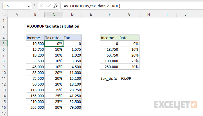
In the worksheet shown, the formula in cell C5 is:
=VLOOKUP(B5,tax_data,2,TRUE)
VLOOKUP requires lookup values to be in the first column of the lookup table. To retrieve the correct tax rate for the income in column B, VLOOKUP is configured like this:
- The lookup_value comes from cell B5
- The table_array is the named range tax_data (F5:G9)
- The col_index_num is 2 since the tax rates are in the second column of tax_data
- The range_lookup argument is set to TRUE = approximate match
With this configuration, VLOOKUP scans the lookup values until it finds a value greater than the value in B5, then VLOOKUP "drops back" to the previous row and returns the corresponding tax rate from that row. Because we are using VLOOKUP in approximate match mode, with range_lookup set to TRUE, the lookup values in F5:F9 must be sorted in ascending order.
As the formula is copied down column C, the VLOOKUP function looks up the income in column B in the range F5:F9 and returns the correct tax rate from the range G5:G9. A formula in column D multiples the income by the tax rate to display the total tax amount.
Note: this formula calculates a tax rate in a simple one-tier scheme. To calculate tax based on a progressive system where income is taxed at different rates in multiple tiers, see this example.
Named range optional
The named range in this example is optional and used for convenience only because it makes the formula easier to read and means that the tax rate does not need to be locked. To avoid a named range, use an absolute reference like this:
=VLOOKUP(B5,$F$5:$G$9,2,TRUE)
VLOOKUP match modes
VLOOKUP has two match modes: exact match and approximate match, controlled by an optional fourth argument called range_lookup. When range_lookup is omitted, it defaults to TRUE and VLOOKUP performs an approximate match. This means we could leave out the last argument and get the same result:
=VLOOKUP(B5,tax_data,2)
However, in this example, the fourth argument has been set to TRUE explicitly for clarity. For a complete overview of VLOOKUP with many examples see our VLOOKUP page.
Note: I think the default behavior of VLOOKUP is dangerous because it can easily produce incorrect results that look normal. For that reason, I recommend that you always provide a value for range_lookup as a reminder to yourself and others of the behavior you intend.
Total tax
The tax rates in column D are decimal values formatted with the percentage number format. The formula to calculate the total tax in cell D5 multiples Income by the Tax rate:
=B5*C5
As the formula is copied down, it returns the total tax for each row in the data.