Summary
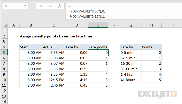
To assign penalty points based on an amount of time late, you can use a nested IF formula.In the example shown, the formula in E5 is:
=
IF(D5<VALUE("0:05"),0,
IF(D5<VALUE("0:15"),1,
IF(D5<VALUE("0:30"),2,
IF(D5<VALUE("0:60"),3,
IF(D5<VALUE("4:00"),4,
5)))))
Note: line breaks added for readability.
Generic formula
=
IF(time<VALUE("0:05"),0,
IF(time<VALUE("0:15"),1,
IF(time<VALUE("0:30"),2,
IF(time<VALUE("0:60"),3,
IF(time<VALUE("4:00"),4,
5)))))
Explanation
This formula is a classic example of a nested IF formula that tests threshold values in ascending order. To match the schedule shown in G5:G11, the formula first checks the late by time in D5 to see if it's less than 5 minutes. If so, zero points are assigned:
IF(D5<VALUE("0:05"),0,
If the result of the logical test above is FALSE, the formula checks to see if D5 is less than the next threshold, which is 15 minutes:
IF(D5<VALUE("0:15"),1,
The same pattern repeats at each threshold. Because the tests are run in order, from smallest to largest, there is no need for more complicated bracketing.
The VALUE function is used to make Excel treat time value at each threshold as a number instead of next.
Note: you can also use VLOOKUP to replace nested IFs if you like.