Summary
Number formats are a key feature in Excel. Their key benefit is that they change how numeric values look without actually changing any data. Excel ships with a huge number of different number formats, and you can easily define your own. This guide explains how custom number formats work in detail.
Introduction
Number formats control how numbers are displayed in Excel. The key benefit of number formats is that they change how a number looks without changing any data. They are a great way to save time in Excel because they perform a huge amount of formatting automatically. As a bonus, they make worksheets look more consistent and professional.
Video: What is a number format
What can you do with custom number formats?
Custom number formats can control the display of numbers, dates, times, fractions, percentages, and other numeric values. Using custom formats, you can do things like format dates to show month names only, format large numbers in millions or thousands, and display negative numbers in red.
Where can you use custom number formats?
Many areas in Excel support number formats. You can use them in tables, charts, pivot tables, formulas, and directly on the worksheet.
- Worksheet - format cells dialog
- Pivot Tables - via value field settings
- Charts - data labels and axis options
- Formulas - via the TEXT function
What is a number format?
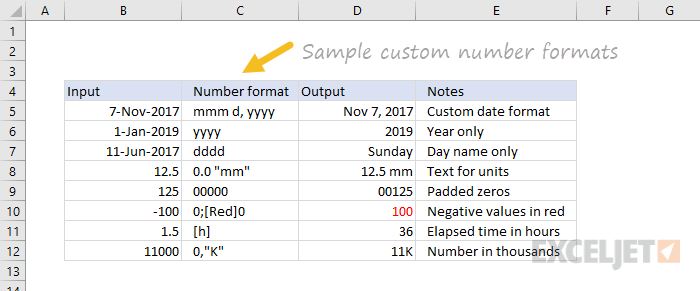
A number format is a special code to control how a value is displayed in Excel. For example, the table below shows 7 different number formats applied to the same date, January 1, 2019:
| Input | Code | Result |
|---|---|---|
| 1-Jan-2019 | yyyy | 2019 |
| 1-Jan-2019 | yy | 19 |
| 1-Jan-2019 | mmm | Jan |
| 1-Jan-2019 | mmmm | January |
| 1-Jan-2019 | d | 1 |
| 1-Jan-2019 | ddd | Tue |
| 1-Jan-2019 | dddd | Tuesday |
The key thing to understand is that number formats change the way numeric values are displayed, but they do not change the actual values.
Where can you find number formats?
On the home tab of the ribbon, you'll find a menu of built-in number formats. Below this menu to the right, there is a small button to access all number formats, including custom formats:
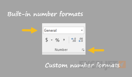
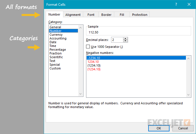
This button opens the Format Cells dialog box. You'll find a complete list of number formats, organized by category, on the Number tab:
Note: You can open the Format Cells dialog box with the keyboard shortcut Control + 1.
General is the default
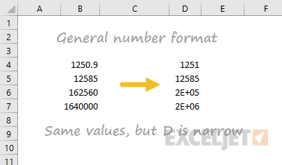
By default, cells start with the General format applied. The display of numbers using the General number format is somewhat "fluid". Excel will display as many decimal places as space allows, and will round decimals and use scientific number format when space is limited. The screen below shows the same values in columns B and D, but D is narrower and Excel makes adjustments on the fly.
How to change number formats
You can select standard number formats (General, Number, Currency, Accounting, Short Date, Long Date, Time, Percentage, Fraction, Scientific, Text) on the home tab of the ribbon using the Number Format menu.
Note: As you enter data, Excel will sometimes change number formats automatically. For example, if you enter a valid date, Excel will change to "Date" format. If you enter a percentage like 5%, Excel will change to Percentage, and so on.
Shortcuts for number formats
Excel provides a number of keyboard shortcuts for some common formats:
| Format | Shortcut |
|---|---|
| General format | Ctrl Shift ~ |
| Currency format | Ctrl Shift $ |
| Percentage format | Ctrl Shift % |
| Scientific format | Ctrl Shift ^ |
| Date format | Ctrl Shift # |
| Time format | Ctrl Shift @ |
| Custom formats | Control + 1 |
See also: 222 Excel Shortcuts for Windows and Mac | The Excel shortcuts you really should know
Where to enter custom formats
At the bottom of the predefined formats, you'll see a category called custom. The Custom category shows a list of codes you can use for custom number formats, along with an input area to enter codes manually in various combinations.
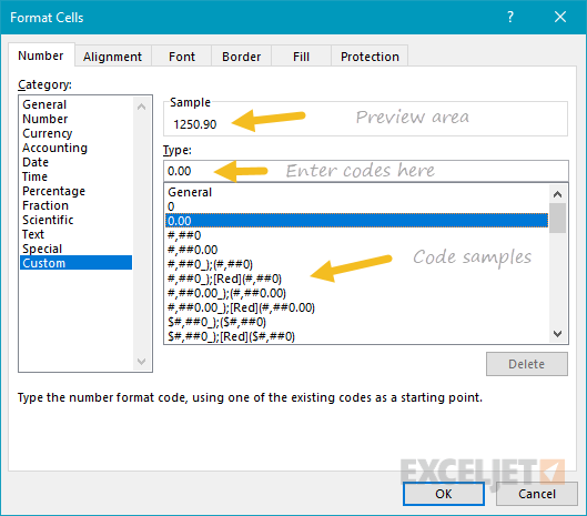
When you select a code from the list, you'll see it appear in the Type input box. Here you can modify existing custom code or enter your own code from scratch. Excel will show a small preview of the code applied to the first selected value above the input area.
Note: Custom number formats live in a workbook, not in Excel generally. If you copy a value formatted with a custom format from one workbook to another, the custom number format will be transferred into the workbook along with the value.
How to create a custom number format
To create a custom number format, follow this simple 4-step process:
- Select cell(s) with values you want to format
- Control + 1 > Numbers > Custom
- Enter codes and watch the preview area to see the result
- Press OK to save and apply
Tip: if you want to base your custom format on an existing format, first apply the base format, then click the "Custom" category and edit codes as you like.
How to edit a custom number format
You can't really edit a custom number format per se. When you change an existing custom number format, a new format is created and will appear in the list in the Custom category. You can use the Delete button to delete custom formats you no longer need.
Warning: there is no "undo" after deleting a custom number format!
Structure and Reference
Excel custom number formats have a specific structure. Each number format can have up to four sections, separated by semi-colons as follows:
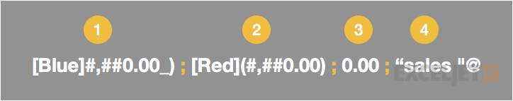
This structure can make custom number formats look overwhelmingly complex. To read a custom number format, learn to spot the semi-colons and mentally parse the code into these sections:
- Positive values
- Negative values
- Zero values
- Text values
Not all sections are required
Although a number format can include up to four sections, only one section is required. By default, the first section applies to positive numbers, the second section applies to negative numbers, the third section applies to zero values, and the fourth section applies to text.
- When only one format is provided, Excel will use that format for all values.
- If you provide a number format with just two sections, the first section is used for positive numbers and zeros, and the second section is used for negative numbers.
- To skip a section, include a semi-colon in the proper location, but don't specify a format code.
Characters that display natively
Some characters appear normally in a number format, while others require special handling. The following characters can be used without any special handling:
| Character | Comment |
|---|---|
| $ | Dollar |
| +- | Plus, minus |
| () | Parentheses |
| {} | Curly braces |
| <> | Less than, greater than |
| = | Equal |
| : | Colon* |
| ^ | Caret |
| ' | Apostrophe |
| / | Forward slash* |
| ! | Exclamation point |
| & | Ampersand |
| ~ | Tilde |
| Space character |
- Update December 2023: The colon (:) and forward slash (/) used to work natively but now must be escaped.
Escaping characters
Some characters won't work correctly in a custom number format without being escaped. For example, the asterisk (*), hash (#), and percent (%) characters can't be used directly in a custom number format – they won't appear in the result. The escape character in custom number formats is the backslash (). By placing the backslash before the character, you can use it in custom number formats:
| Value | Code | Result |
|---|---|---|
| 100 | #0 | #100 |
| 100 | *0 | *100 |
| 100 | %0 | %100 |
Placeholders
Certain characters have a special meaning in custom number format codes. The following characters are key building blocks:
| Character | Purpose |
|---|---|
| 0 | Display insignificant zeros |
| # | Display significant digits |
| ? | Display aligned decimals |
| . | Decimal point |
| , | Thousands separator |
| * | Repeat the following character |
| _ | Add space |
| @ | Placeholder for text |
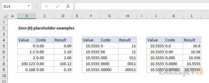
Zero (0) is used to force the display of insignificant zeros when a number has fewer digits than zeros in the format. For example, the custom format 0.00 will display zero as 0.00, 1.1 as 1.10, and .5 as 0.50.
Pound sign (#) is a placeholder for optional digits. When a number has fewer digits than # symbols in the format, nothing will be displayed. For example, the custom format #.## will display 1.15 as 1.15 and 1.1 as 1.1.
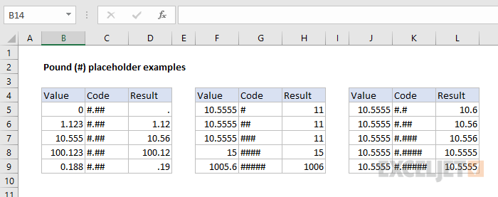
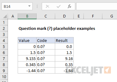
Question mark (?) is used to align digits. When a question mark occupies a place not needed in a number, a space will be added to maintain visual alignment.
Period (.) is a placeholder for the decimal point in a number. When a period is used in a custom number format, it will always be displayed, regardless of whether the number contains decimal values.
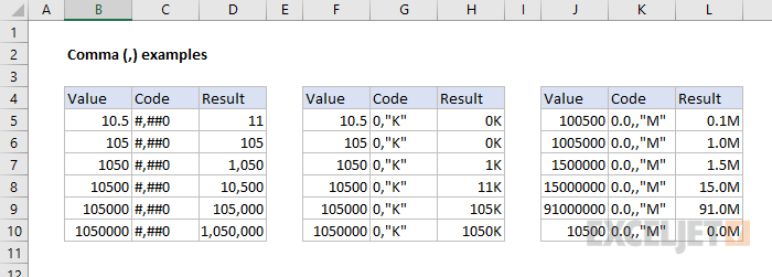
Comma (,) is a placeholder for the thousands separator in the number being displayed. It can be used to define the behavior of digits in relation to the thousands or millions digits.
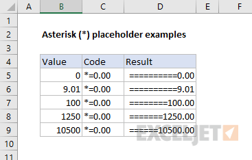
Asterisk (*) is used to repeat characters. The character immediately following an asterisk will be repeated to fill the remaining space in a cell.
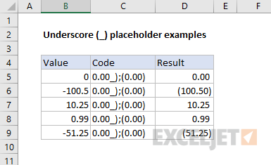
Underscore (_) is used to add space in a number format. The character immediately following an underscore character controls how much space to add. A common use of the underscore character is to add space to align positive and negative values when a number format adds parentheses to negative numbers only. For example, the number format "0_);(0)" adds a bit of space to the right of positive numbers so that they stay aligned with negative numbers, which are enclosed in parentheses.
At (@) - placeholder for text. For example, the following number format will display text values in blue:
0;0;0;[Blue]@
See below for more information about using color.
Automatic rounding
It's important to understand that Excel will perform "visual rounding" with all custom number formats. When a number has more digits than placeholders on the right side of the decimal point, the number is rounded to the number of placeholders. When a number has more digits than placeholders on the left side of the decimal point, extra digits are displayed. This is a visual effect only; actual values are not modified.
Number formats for TEXT
To display text together with numbers, enclose the text in double quotes (""). You can use this approach to append or prepend text strings in a custom number format, as shown in the table below.
| Value | Code | Result |
|---|---|---|
| 10 | General" units" | 10 units |
| 10 | 0.0" units" | 10.0 units |
| 5.5 | 0.0" feet" | 5.5 feet |
| 30000 | 0" feet" | 30000 feet |
| 95.2 | "Score: "0.0 | Score: 95.2 |
| 1-Jun | "Date: "mmmm d | Date: June 1 |
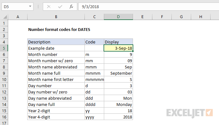
Number formats for DATES
Dates in Excel are just numbers, so you can use custom number formats to change how they are displayed. Excel has many specific codes you can use to display components of a date in different ways. The screen below shows how Excel displays the date in D5, September 3, 2018, with a variety of custom number formats:
Number formats for TIME
Times in Excel are fractional parts of a day. For example, 12:00 PM is 0.5, and 6:00 PM is 0.75. You can use the following codes in custom time formats to display components of a time in different ways. The screen below shows how Excel displays the time in D5, 9:35:07 AM, with a variety of custom number formats:
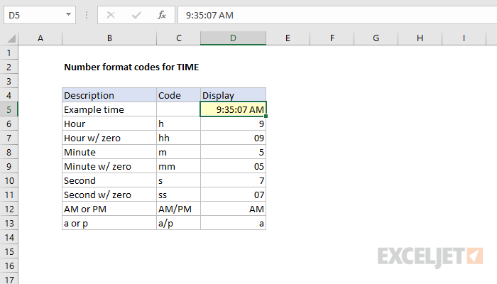
Note: m and mm can't be used alone in a custom number format since they conflict with the month number code in date format codes.
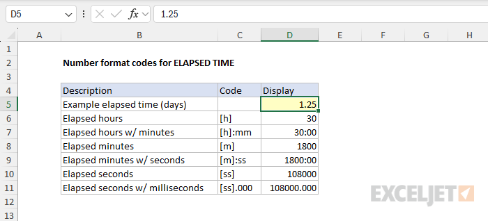
Number formats for ELAPSED TIME
Elapsed time is a special case and needs special handling. By using square brackets, Excel provides a special way to display elapsed hours, minutes, and seconds. The following screen shows how Excel displays elapsed time based on the value in D5, which represents 1.25 days:
Number formats for fractional seconds
The following custom number formats will display tenths, hundredths, or thousandths of a second:
mm:ss.0 // tenths of a second (deciseconds)
mm:ss.00 // hundredths of a second (centiseconds)
mm:ss.000 // thousandths of a second (milliseconds)
For a full write-up on working with fractional seconds in Excel, see this article.
Number formats for COLORS
Excel provides basic support for colors in custom number formats. The following 8 colors can be specified by name in a number format: [black] [white] [red][green] [blue] [yellow] [magenta] [cyan]. Color names must appear in brackets.
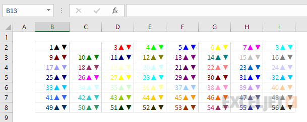
Colors by index
In addition to color names, it's also possible to specify colors by an index number (Color1, Color2, Color3, etc.) The examples below are using the custom number format: [ColorX]0"▲▼", where X is a number between 1 and 56:
[Color1]0"▲▼" // black
[Color2]0"▲▼" // white
[Color3]0"▲▼" // red
[Color4]0"▲▼" // green
etc.
You may need to adjust the name "Color" for other regions or locales. For example, use [ColourX] instead of [ColorX] on a system using British English.
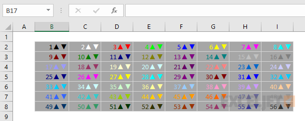
The triangle symbols have been added only to make the colors easier to see. The first image shows all 56 colors on a standard white background. The second image shows the same colors on a gray background. Note that the first 8 colors shown correspond to the named color list above.
Apply number formats in a formula
Although most number formats are applied directly to cells in a worksheet, you can also apply number formats inside a formula with the TEXT function. For example, with a valid date in A1, the following formula will display the month name only:
=TEXT(A1,"mmmm")
The result of the TEXT function is always text, so you are free to concatenate the result of TEXT to other strings:
="The contract expires in "&TEXT(A1,"mmmm")
The screen below shows the number formats in column C being applied to numbers in column B using the TEXT function:
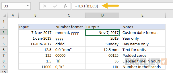
One quirk of the TEXT function relates to double quotes ("") that are part of certain custom number formats. Because the format_text is entered as a text string, Excel won't allow you to enter the formula without removing the quotes or adding more quotes. For example, to display a large number in thousands, you can use a custom number format like this:
0, "k"
Notice that k appears in quotes ("k"). To apply the same format with the TEXT function, you can use:
=TEXT(A1,"0, k")
Notice the k is not surrounded by quotes. Alternatively, you can add extra double quotes as below, which returns the same result:
=TEXT(A1,"0,""K""")
This behavior only occurs when you are hardcoding a format inside TEXT. If you are applying a format entered elsewhere on the worksheet (as in cells C6 and C9 in the worksheet above) you can use a standard number format.
Measurements
You can use a custom number format to display numbers with an inch mark (") or a feet mark ('). In the screen below, the number formats used for inches and feet are:
0.00 \' // feet
0.00 \" // inches
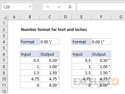
These results are simplistic and can't be combined in a single number format. You can, however, use a formula to display feet together with inches.
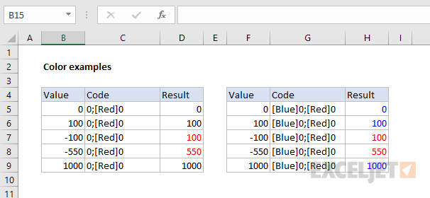
Conditionals
Custom number formats can apply up to two conditions, which are written in square brackets like [>100] or [<=100]. When you use conditionals in custom number formats, you override the standard [positive];[negative];[zero];[text] structure. For example, to display values below 100 in red, you can use:
[Red][<100]0;0
To display values greater than or equal to 100 in blue, you can extend the format like this:
[Red][<100]0;[Blue][>=100]0
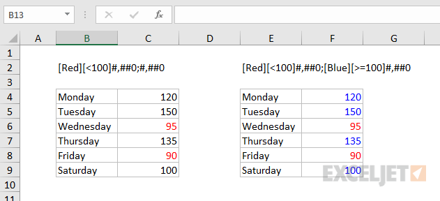
To apply more than two conditions, or to change other cell attributes, like fill color, etc., you'll need to switch to Conditional Formatting, which can apply formatting with much more power and flexibility using formulas.
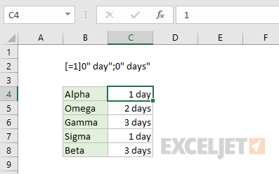
Plural text labels
You can use conditionals to add an "s" to labels greater than zero with a custom format like this:
[=1]0" day";0" days"
Telephone numbers
Custom number formats can also be used for telephone numbers, as shown in the screen below:
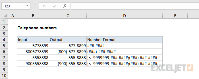
Notice that the third and fourth examples use a conditional format to check for numbers that contain an area code. If you have data that contains phone numbers with hard-coded punctuation (parentheses, hyphens, etc.) you will need to clean the telephone numbers first so that they only contain numbers.
Hide all content
You can use a custom number format to hide all content in a cell. The code is simply three semi-colons and nothing else ;;;
To reveal the content again, you can use the keyboard shortcut Control + Shift + ~, which applies the General format.
Other resources
- Developer Bryan Braun built a nice interactive tool for building custom number formats


