Ever use Excel's MOD function?
The MOD function performs the modulo operation. It takes a number and a divisor, does the division, and gives you back the remainder.
Unless you're a programmer, this might seem way too nerdy. Modulo? Seriously? What can the average person do with that?
As it turns out — a lot!
Note: MOD turns up in many compact, elegant formulas in Excel. In fact, if you use MOD in one of your formulas, people will automatically assume you're an Excel pro, so take care :)
To illustrate how MOD is useful, let me pose a simple problem:
Let's say you maintain a budget with some monthly expenses, and you'd like to enter an expense that occurs every 3 months, and zero for months in between. You want something like this:

Simple, right? But how to begin...what kind of formula does something every 3 months?
Believe it or not, the MOD function is the key.
Earlier, I mentioned the remainder. The trick in this case is not the remainder itself, but rather what it means when you don't get a remainder. In other words, when MOD returns zero.
Think about it — when the remainder is zero, it means the divisor goes into the number evenly.
Hmmm...we can use that!
Note: if you want more background on why MOD works well for repeating things, Khan Academy has a nice explanation of modular arithmetic.
We want to do something every 3 months. So, if we run the month number through MOD with a divisor of 3, and get zero as the result, it's time to add the expense.
Let's do it.
First, let's add month numbers above our table so we have something to work with right away.
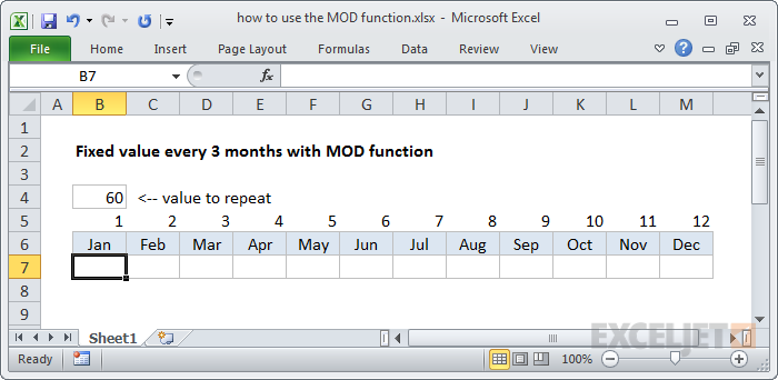
Tip: When you're building a more complex formula, don't be afraid to hard-code values that will help you validate your ideas quickly. Think of this as rapid prototyping. Once you know your approach will work, you can come back and figure out how to remove the hard-coded values. Don't optimize prematurely!
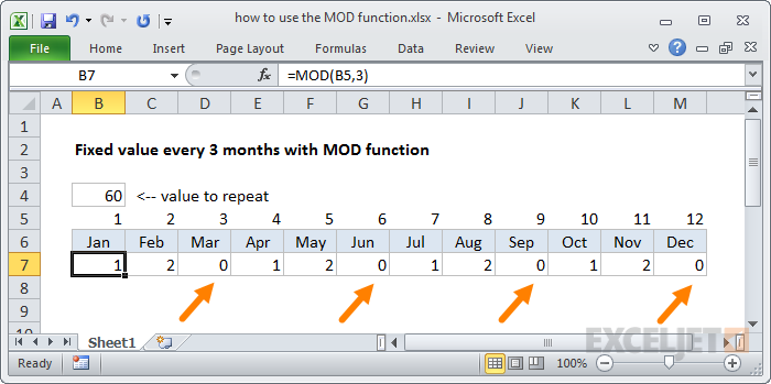
Now, with the month numbers in place, we'll enter a simple MOD formula.
=MOD(B5,3)
This gives us the remainder in each cell, and every 3 months, we get a remainder of zero.
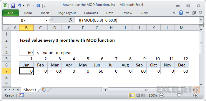
Next, let's get our value in there when the remainder is zero, and get rid of the other numbers. We can do this by adding an IF statement to test for a zero remainder: if the remainder is zero, return 60, otherwise return 0.
=IF(MOD(B5,3)=0,60,0)
Now we have 60 at every 3rd month and a zero in between. Cool.
Next, we'll replace the hardcoded 60 with a reference to B4 so we can easily change it later. Obviously, if the value will never change, there's no need to do this, but it's a good practice to expose inputs on the worksheet, especially when they appear in more than one place, and might change later.
We use an absolute reference for B4 so we can copy the formula across without it changing.
=IF(MOD(B5,3)=0,$B$4,0)
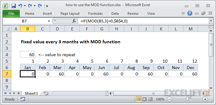
This is just what we need, but it's time to get rid of those unsightly numbers we added above the months.
How can we do it?
There are two ways we can deal with this. One method uses the COLUMN function, and one uses the MONTH function. (See how knowing more Excel functions can be useful?)
We'll look at COLUMN first...
With the COLUMN function
The COLUMN function returns the column number of a given reference. When you don't give COLUMN a reference, it returns the column number of the current cell. This is easier to show than explain, so let's add the COLUMN function to the cells that currently contain month numbers:
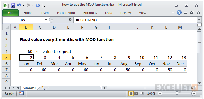
This is nice, but notice that it's not quite what we need. The first number starts with 2, not 1, because the first formula sits in the second column. So this throws off our repeating values.
Easily solved. We just need to subtract 1 from the column number:
COLUMN()-1
Note: think of 1 as an "offset" that you adjust as needed for your situation.
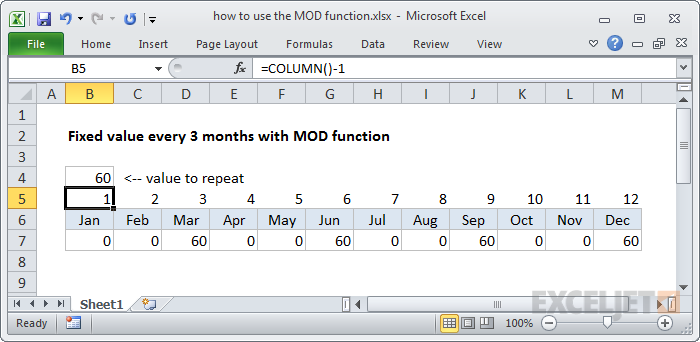
Now COLUMN generates the month numbers we need, and we can update our formula. We simply nest the COLUMN function where we had a reference to the month numbers:
=IF(MOD(COLUMN()-1,3)=0,$B$4,0)
Then we can delete the numbers:
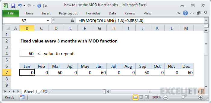
With the MONTH function
While the COLUMN function works fine, it's a little awkward, because we have to hardcode an offset value to get a correct month number. We only have 12 months — isn't there some way to use the month numbers directly? Yes, in fact, there is.
With a little tweak, we can build a more logical formula by using actual dates. To do this, we need to replace the month abbreviations ("Jan", "Feb", "Mar", etc.) with full dates like 1/1/2016, 2/1/2016, 3/1/2016, etc.
Tip: Enter the first two dates then select them both, and use the fill handle to have Excel fill in the rest.
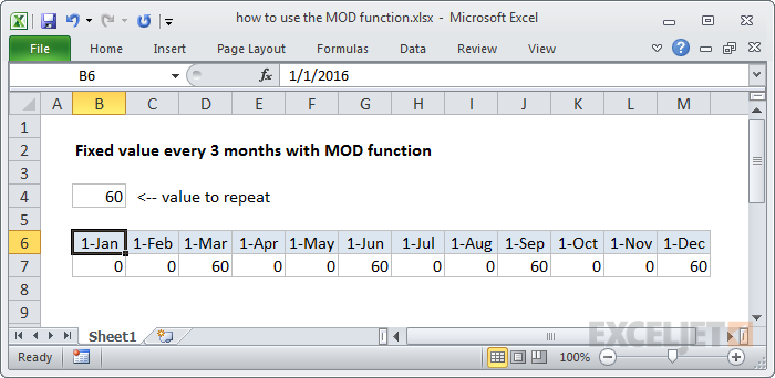
At first, this looks silly — people don't want to see actual dates for months.
No problem. All we need to do is apply the custom number format "mmm" to the dates, and we've got abbreviated month names again:

Same dates with the custom date format "ddd".
The beauty of this approach is that the column headers now contain regular dates, so we can use normal date functions on them.
And now we can simply use the MONTH function to get the number, and ditch COLUMN:
=IF(MOD(MONTH(B6),3)=0,$B$4,0)
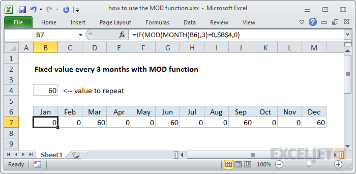
This eliminates that offset value, and the formula will work wherever the budget table appears in the worksheet.
More MOD formulas
As I mentioned, the MOD function is a versatile function and can be used in many ways, so you'll see it in a variety of formulas. It's particularly useful for "every nth" type formulas, but it's handy for other things to. Here's a list of examples you can use for inspiration.
Sum every nth column
Extract time from a date and time
Count cells that contain odd numbers
Convert time to time zone
Highlight integers only
Fixed value every N months
Highlight every other row
Calculate elapsed work time
More Excel formulas and functions
If you want to master more Excel formulas and functions, we have some good resources for you:


