
Summary
Many Excel experts believe that Pivot Tables are the single most powerful tool in Excel. This article provides more than 20 tips you should know to work productively with Excel Pivot Tables.
Quick Links
Pivot tables are a reporting engine built into Excel. They are the single best tool in Excel for analyzing data without formulas. You can create a basic pivot table in about one minute and begin interactively exploring your data. Below are more than 20 tips for getting the most from this flexible and powerful tool.
1. You can build a pivot table in about one minute
Many people think building a pivot table is complicated and time-consuming, but it's simply not true. Compared to the time it would take you to build an equivalent report manually, pivot tables are incredibly fast. If you have well-structured source data, you can create a pivot table in less than a minute. Start by selecting any cell in the source data:
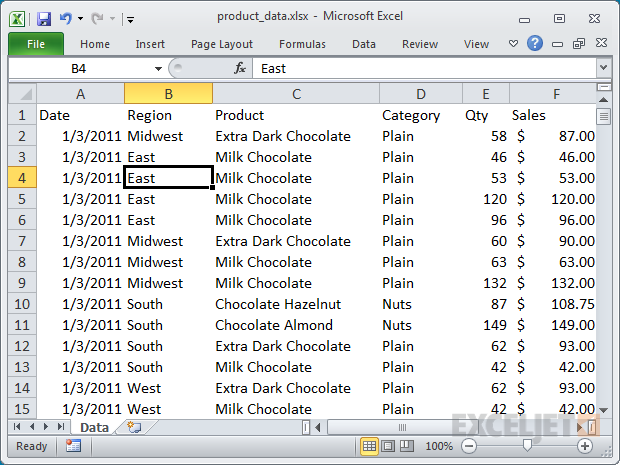
Example source data
Next, follow these four steps:
- On the Insert tab of the ribbon, click the PivotTable button
- In the Create PivotTable dialog box, check the data and click OK
- Drag a "label" field into the Row Labels area (e.g. customer)
- Drag a numeric field into the Values area (e.g. sales)
A basic pivot table in about 30 seconds
The pivot table above shows total sales by product, but you can easily rearrange fields to show total sales by region, by category, by month, and so on. Watch the video below for a quick demonstration:
Video: How to quickly create a pivot table
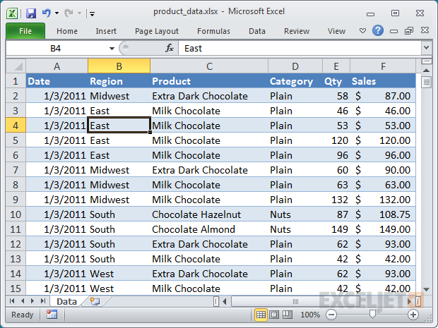
2. Clean your source data
To minimize problems down the road, make sure your data is in good shape. Source data should have no blank rows or columns, and no subtotals. Each column should have a unique name (on one row only) and represent a field for each row/record in the data:
Perfect data for a pivot table!
You might sometimes need to add missing data. See this video for tips:
Video: How to quickly fill in missing data
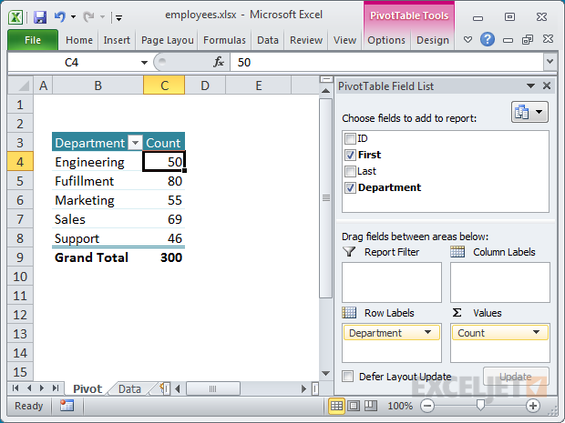
3. Count the data first
When you first create a pivot table, use it to generate a simple count first to make sure the pivot table is processing the data as you expect. To do this, simply add any text field as a Value field. You'll see a very small pivot table that displays the total record count, that is, the total number of rows in your data. If this number makes sense to you, you're good to go. If the number doesn't make sense to you, it's possible the pivot table is not reading the data correctly or that the data has not been defined correctly.
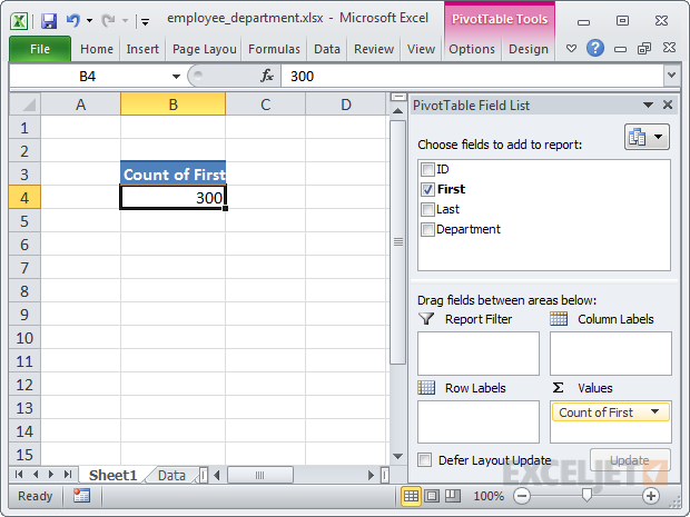
300 first names means we have 300 employees. Check.
4. Plan before you build
Although it's a lot of fun dragging fields around a pivot table and watching Excel churn out yet another unusual representation of the data, you can find yourself going down a lot of unproductive rabbit holes very easily. An hour later, it's not so fun anymore. Before you start building, jot down what you are trying to measure or understand, and sketch out a few simple reports on a notepad. These simple notes will help guide you through the huge number of choices you have at your disposal. Keep things simple, and focus on the questions you need to answer.
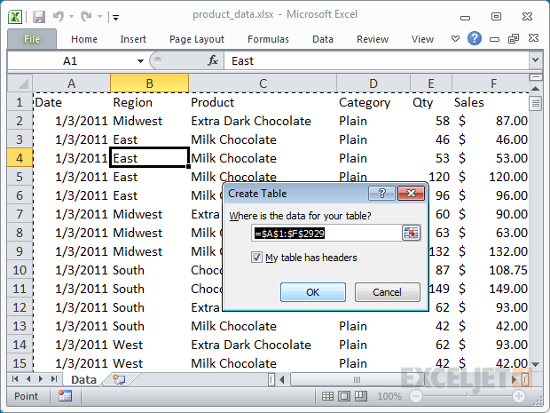
5. Use a table for your data to create a "dynamic range"
If you use an Excel Table for the source data of your pivot table, you get a very nice benefit: your data range becomes "dynamic". A dynamic range will automatically expand and shrink the table as you add or remove data, so you won't have to worry that the pivot table is missing the latest data. When you use a Table for your pivot table, the pivot table will always be in sync with your data.
To use a Table for your pivot table:
- Select any cell in the data and use the keyboard shortcut Ctrl-T to create a Table
- Click the Summarize with PivotTable button (TableTools > Design)
- Build your pivot table normally
- Profit: data you add to your Table will automatically appear in your Pivot table on refresh
Video: Use a table for your next pivot table
Creating a simple Table from the data using (Ctrl-T)
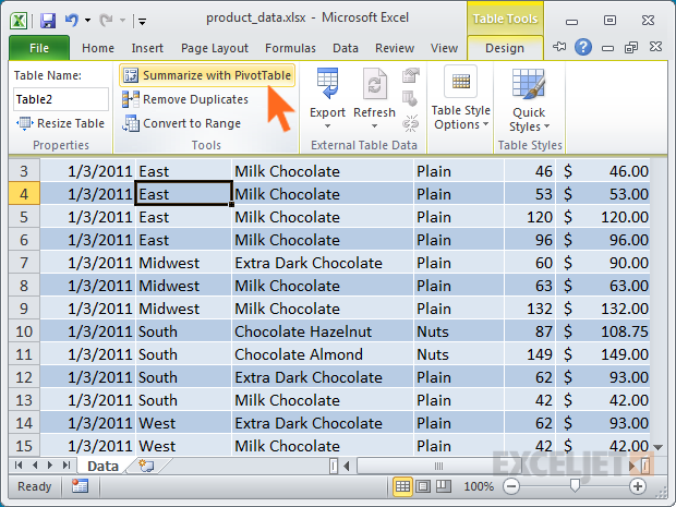
Now that we have a table, we can use Summarize with a Pivot Table
Still need inspiration on why you should learn pivot tables? See my personal story.
6. Use a pivot table to count things
By default, a Pivot Table will count any text field. This can be a really handy feature in a lot of general business situations. For example, suppose you have a list of employees and want to get a count by department. To get a breakdown by department, follow these steps:
- Create a pivot table normally
- Add the Department as a Row Label
- Add the employee Name field as a Value
- The pivot table will display a count of employees by Department
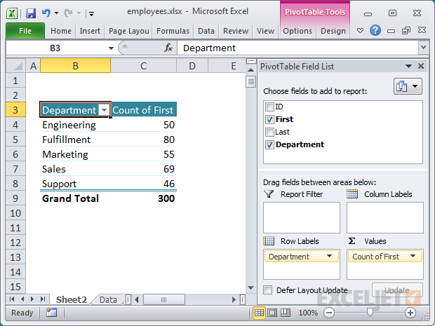
Employee breakdown by department
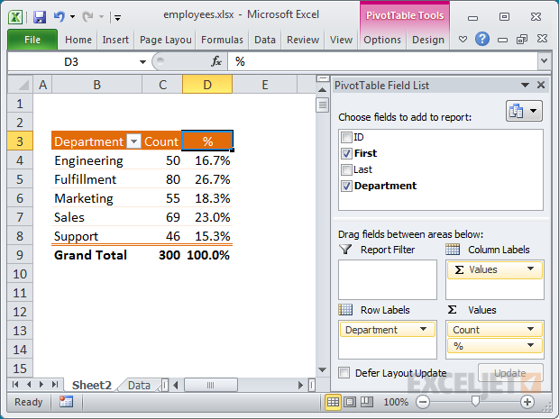
7. Show totals as a percentage
In many pivot tables, you'll want to show a percentage rather than a count. For example, perhaps you want to show a breakdown of sales by product. But, rather than show the total sales for each product, you want to show sales as a percentage of the total sales. Assuming you have a field called Sales in your data, just follow these steps:
- Add Product to the pivot table as a Row Label
- Add Sales to the pivot table as a Value
- Right-click the Sales field, and set "Show Values As" to "% of Grand Total"
See the tip below, "Add a field more than once to a pivot table," to learn how to show total sales and sales as a percent of total at the same time.
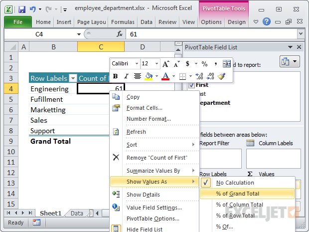
Changing value display to % of total
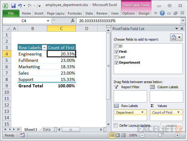
The sum of employees displayed as % of total
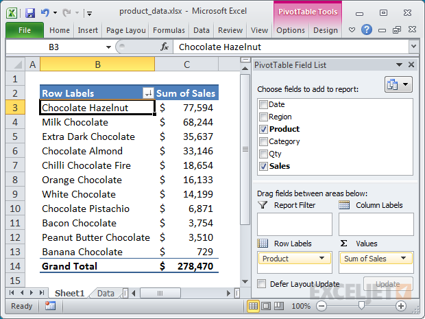
8. Use a pivot table to build a list of unique values
Because pivot tables summarize data, they can be used to find unique values in a field. This is a good way to quickly see all the values that appear in a field and also find typos and other inconsistencies. For example, suppose you have sales data, and you want to see a list of every product that was sold. To create a product list:
- Create a pivot table normally
- Add the Product as a Row Label
- Add any other text field (category, customer, etc) as a Value
- The pivot table will show a list of all products that appear in the sales data
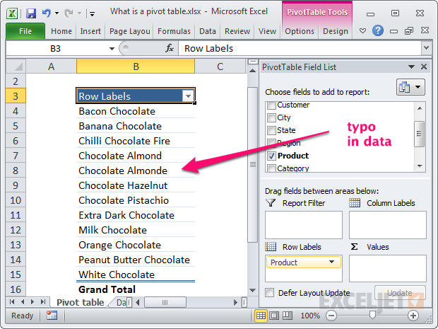
Every product that appears in the data is listed (including a typo)
If you need more structured learning, we have a nice course on Pivot Tables.
9. Create a self-contained pivot table
When you've created a pivot table from data in the same worksheet, you can remove the data if you like, and the pivot table will continue to operate normally. This is because a pivot table has a pivot cache that contains an exact duplicate of the data used to create the pivot table.
- Refresh the pivot table to ensure the cache is up to date (PivotTable Tools > Refresh)
- Delete the worksheet that contains the data
- Use your pivot table normally
Video: How to make a self-contained pivot table
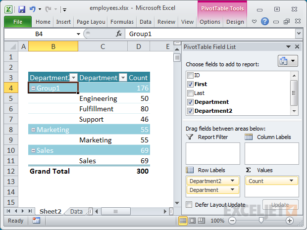
10. Group a pivot table manually
Although pivot tables automatically group data in many ways, you can also group items manually into your own custom groups. For example, assume you have a pivot table that shows a breakdown of employees by department. Suppose you want to further group the Engineering, Fulfillment, and Support departments into Group 1, and Sales and Marketing into Group 2. Group 1 and Group 2 don't appear in the data; they are your own custom groups. To group the pivot table into the ad hoc groups, Group 1 and Group 2:
- Control-click to select each item in the first group
- Right-click one of the items and choose Group from the menu
- Excel creates a new group, "Group1"
- Select Marketing and Sales in column B, and group as above
- Excel creates another group, "Group2"
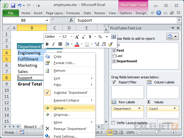
Starting to group manually
Half way through manual grouping - Group 1 is done
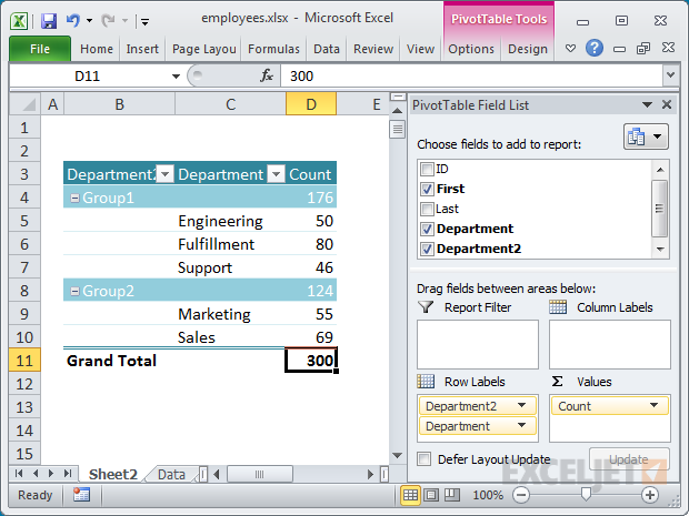
Finished grouping manually
11. Group numeric data into ranges
One of the most interesting and powerful features that every pivot table has is the ability to group numeric data into ranges or buckets. For example, assume you have a list of voting results that includes voter age, and you want to summarize the results by age group:
- Create your pivot table normally
- Add Age as a Row Label, Vote as a Column Label, and Name as a Value
- Right-click any value in the Age field and choose Group
- Enter 10 as the interval in the "By:" input area
- When you click OK, you'll see the voting data grouped by age into 10-year buckets
Video: How to group a pivot table by age range
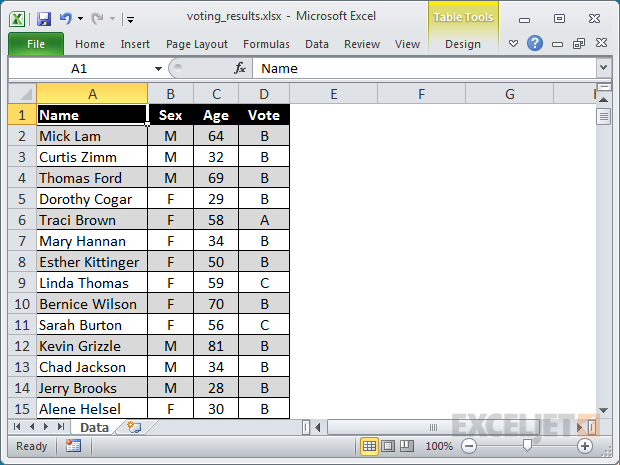
The source data for voting results
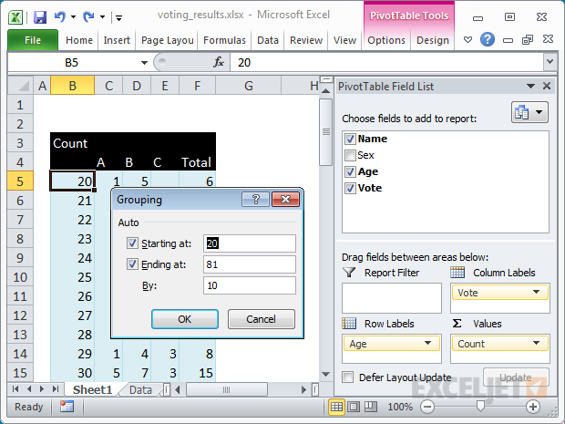
Grouping the age field into 10-year buckets
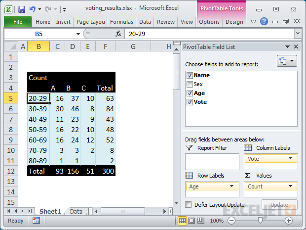
Done grouping voting results by age range
12. Rename fields for better readability
When you add fields to a pivot table, the pivot table will display the name that appears in the source data. Value field names will appear with "Sum of " or "Count of" when they are added to a pivot table. For example, you'll see Sum of Sales, Count of Region, and so on. However, you can simply overwrite this name with your own. Just select the cell that contains the field you want to rename and type a new name.
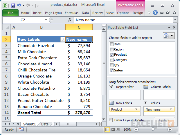
Rename a field by typing over the original name
13. Add a space to field names when Excel complains
When you try to rename fields, you might run into a problem if you try to use exactly the same field name that appears in the data. For example, suppose you have a field called Sales in your source data. As a value field, it appears as Sum of Sales, but (sensibly) you want it to say Sales. However, when you try to use Sales, Excel complains that the field already exists, and throws a "PivotTable field name already exists" error message.
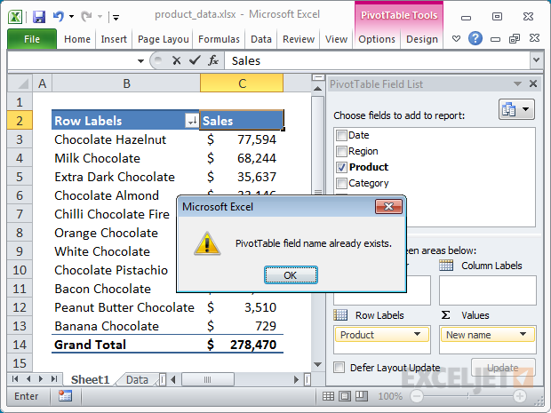
Excel doesn't like your new field name
As a simple workaround, just add a space to the end of your new field name. You can't see a difference, and Excel won't complain.
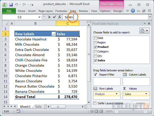
Adding a space to the name avoids the problem
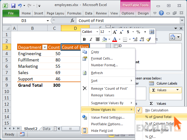
14. Add a field more than once to a pivot table
There are many situations when it makes sense to add the same field to a pivot table more than once. It may seem odd, but you can indeed add the same field to a pivot table more than once. For example, suppose you have a pivot table that shows a count of employees by department.
The count works fine, but you also want to show the count as a percentage of total employees. In this case, the simplest solution is to add the same field twice as a Value field:
- Add a text field to the Value area (e.g., First name, Name, etc.)
- By default, you'll get a count for text fields
- Add the same field again to the Value area
- Right-click the second instance, and change Show Values As to "% of Grand Total"
- Rename both fields as you wish
Setting a field to show percent of total
The Name field has been added twice
15. Automatically format all value fields
Any time you add a numeric field as a Value in a pivot table, you should set the number format directly on the field. You may be tempted to format the values you see in the pivot table directly, but this is not a good idea, because it's not as reliable as the pivot table changes. Setting the format directly on the field will ensure that the field is displayed using the format you want, no matter how big or small the pivot table becomes.
For example, assume a pivot table that shows a breakdown of sales by Region. When you first add the Sales field to the pivot table, it will be displayed in General number format, since it's a numeric field. To apply the Accounting number format to the field itself:
- Right-click on the Sales field and select Value Field Settings from the menu
- Click the Number Format button in the Value field settings dialog that appears
- Set the format to Accounting and click OK to exit
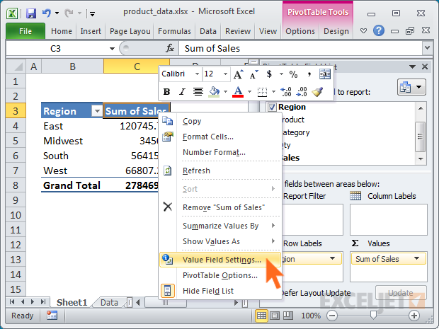
Setting format directly on a value field
16. Drill down to see (or extract) the data behind any total
Whenever you see a total displayed in a pivot table, you can easily see and extract the data that makes up the total by "drilling down". For example, assume you are looking at a pivot table that shows employee count by department. You can see that there are 50 employees in the Engineering department, but you want to see the actual names. To see the 50 people that make up this number, double-click directly on the number 50, and Excel will add a new sheet to your workbook that contains the exact data used to calculate 50 engineers. You can use this same approach to see and extract data behind totals wherever you see them in a pivot table.
Double-click a total to "drill down"
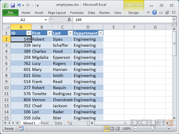
The 50 Engineers, extracted into a new sheet automatically
17. Clone your pivot tables when you need another view
Once you have one pivot table set up, you might want to see a different view of the same data. You could, of course, just rearrange your existing pivot table to create the new view. But if you're building a report that you plan to use and update on an ongoing basis, the easiest thing to do is clone an existing pivot table, so that both views of the data are always available.
There are two easy ways to clone a pivot table. The first way involved duplicating the worksheet that holds the pivot table. If you have a pivot table set up in a worksheet with a title, etc., you can just right-click the worksheet tab to copy the worksheet into the same workbook. Another way to clone a pivot table is to copy the pivot table and paste it somewhere else. Using these approaches, you can make as many copies as you like.
When you clone a pivot table this way, both pivot tables share the same pivot cache. This means that when you refresh any one of the clones (or the original) all of the related pivot tables will be refreshed.
Video: How to clone a pivot table
18. Un-clone a pivot table to refresh independently
After you've cloned a pivot table, you might run into a situation where you really don't want the clone to be linked to the same pivot cache as the original. A common example is after you've grouped a date field in one pivot table, refresh, and discover that you've also accidentally grouped the same date field in another pivot table that you didn't intend to change. When pivot tables share the same pivot cache, they also share field grouping as well.
Here's one way to un-clone a pivot table, that is, unlink it from the pivot cache it shares with other pivot tables in the same worksheet:
- Cut the entire pivot table to the clipboard
- Paste the pivot table into a brand-new workbook
- Refresh the pivot table
- Copy it again to the clipboard
- Paste it back into the original workbook
- Discard the temporary workbook
Your pivot table will now use its own pivot cache and will not refresh with the other pivot table(s) in the workbook, or share the same field grouping.
19. Get rid of useless headings
The default layout for new pivot tables is the Compact layout. This layout will display "Row Labels" and "Column Labels" as headings in the pivot table. These aren't the most intuitive headings, especially for people who don't often use pivot tables. An easy way to get rid of these odd headings is to switch the pivot table layout from Compact to Outline or Tabular layout. This will cause the pivot table to display the actual field names as headings in the pivot table, which is much more sensible. To get rid of these labels altogether, look for a button called Field Headers on the Analyze tab of the Pivot Table Tools ribbon. Clicking this button will disable headings completely.
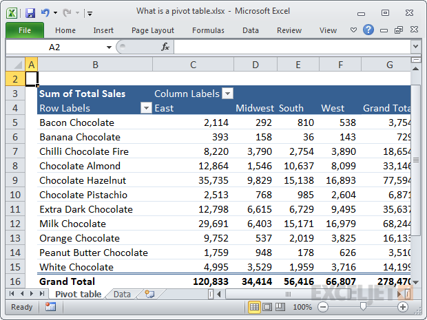
Note the useless and confusing field headings
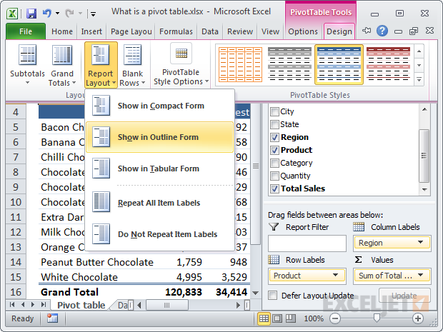
Switching the layout from Compact to Outline
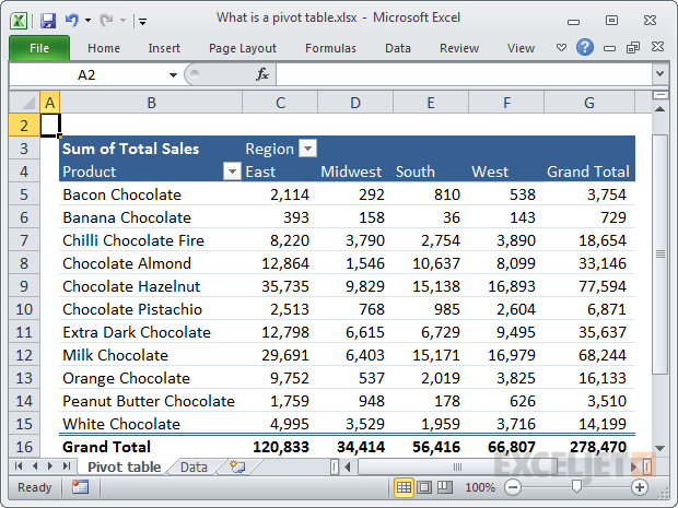
Field headings in the Outline layout are much more sensible
20. Add a little white space around your pivot tables
This is just a simple design tip. All good designers know that a pleasing design requires a little white space. White space just means empty space set aside to give the layout breathing room. After you create a pivot table, insert an extra column to the left and an extra row or two at the top. This will give your pivot table some breathing room and create a better-looking layout. In most cases, I also recommend that you turn off gridlines on the worksheet. The pivot table itself will present a strong visual grid, so the gridlines outside the pivot table are unnecessary, and will simply create visual noise.
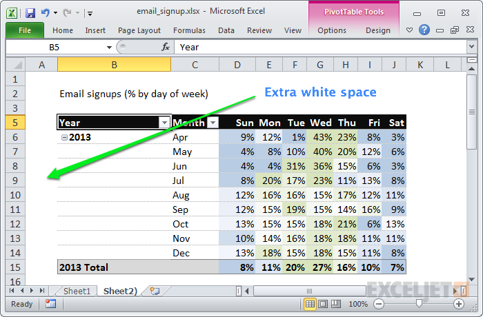
A little white space makes your pivot tables look more polished
Inspiration: 5 pivot tables you haven't seen before.
21. Get rid of row and column grand totals
By default, pivot tables show totals for both rows and columns, but you can easily disable one or both of these totals if you don't want them. On the Pivot Table tab of the ribbon, just click the Totals button and choose the options you want.
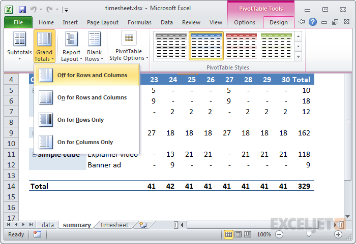
You can remove grand totals for both rows and columns
22. Format empty cells
If you have a pivot table that has a lot of blank cells, you can control the character that is displayed in each blank cell. By default, empty cells will display nothing at all. To set your own character, right-click inside the pivot table and select Pivot Table options. Then make sure that "Empty cells as:" is checked, and enter the character you want to see. Keep in mind that this setting respects the applied number format. For example. If you are using the accounting number format for a numeric value field, and enter a zero, you'll see a hyphen "-" displayed in the pivot table, since that's how zero values are displayed with the Accounting format.
Empty cells set to display 0 (zero) and Accounting number format gives you hyphens
23. Turn off AutoFit when necessary
By default, when you refresh a pivot table, the columns that contain data are adjusted automatically to best fit the data. Normally, this is a good thing, but it can drive you crazy if you have other things on the worksheet along with the pivot table, or if you have carefully adjusted the column widths manually and don't want them changed. To disable this feature, right-click inside the pivot table and choose PivotTable Options. In the first tab of the options (or the layout tab on a Mac), uncheck "AutoFit Column Widths on Update".
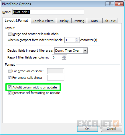
Pivot table column autofit option for Windows
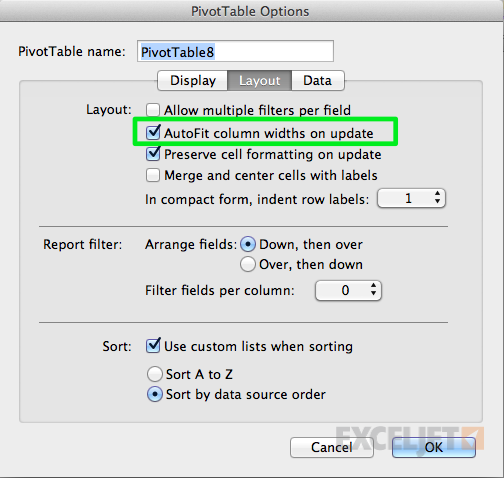
Pivot table column autofit option for Mac
Need to learn more about Pivot Tables? We have solid video training with practice worksheets.


