Pivot table show top 3 values

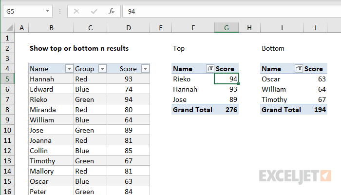
You can use a pivot table to display the top or bottom values in a set of data. In the example shown, one pivot table is used to show the top 3 scores in a set of data, and another pivot table is used to show the bottom 3 values in the same set of data. Because one pivot table was cloned from another, they share the same pivot cache, and both will update when either pivot is refreshed.

How to make this pivot table

1. Create a new pivot table on the same worksheet
2. Add the Name field to the Rows area
3. Add the Score field to the Values area
4. Rename the Score field from "Sum of Score" to "Score " (note trailing space)
5. Filter values to show "Top 3 items by Score"
6. Set sort to "Descending by Score"
7. Copy entire pivot table and paste at cell I4
8. Filter values to show "Bottom 3 items by Score"
9. Set sort to "Ascending by Score"
10. Disable grand totals if desired