Pivot table remove deleted items

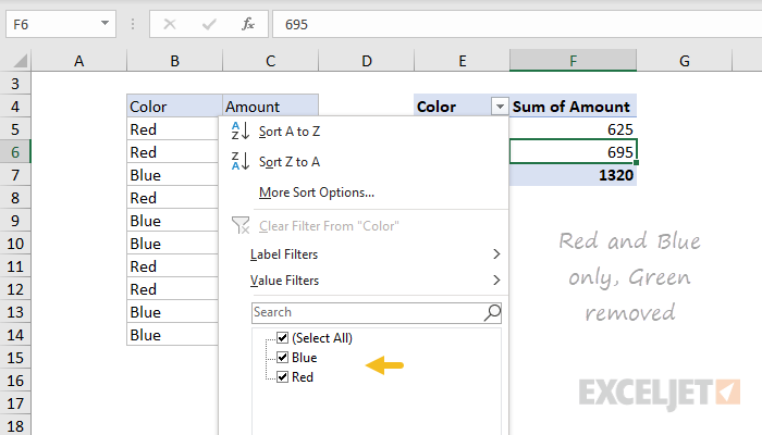
One of the the quirks of pivot tables is that they may hold on to items that have been previously removed from the source data, even after refreshing the data. You may see these deleted "ghost" items when filtering a pivot table. In the example shown, the source data originally contained three colors: red, blue, and green. At some point after the pivot table was created, the color Green disappeared from the source data. However, "Green" still appears when filtering by color in the pivot table.

Remove deleted items from a pivot table

In Excel 2019, and Excel 365, you can remove deleted items by changing a pivot table setting:

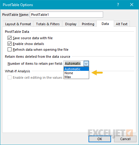
1. Right-click the pivot, select PivotTable Options
   
   


2. Switch to the Data tab
3. Under "Retain items deleted from the data source", select None:
   
   


4. Click OK to exit
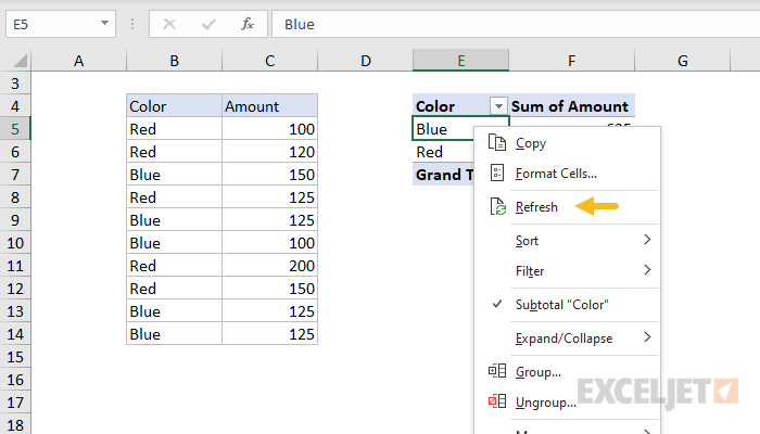
5. Refresh the data
   
   
    
6. Check the filter drop down:
   
   

Set option for all new pivot tables

To change this setting for all new pivot tables:

1. File > Options
2. Data > Data options > Edit Default Layout
3. Pivot Table Options button > Data
4. Set options as above.

Older Excel versions

Older versions of Excel don't have the setting shown above. To remove deleted items, you'll need to use a macro. Debra Dalgleish has a detailed explanation here.