=ACCRINT(id, fd, sd, rate, par, freq, [basis], [calc])- id - Issue date of the security.
- fd - First interest date of security.
- sd - Settlement date of security.
- rate - Interest rate of security.
- par - Par value of security.
- freq - Coupon payments per year (annual = 1, semiannual = 2; quarterly = 4).
- basis - [optional] Day count basis (see below, default =0).
- calc - [optional] Calculation method (see below, default = TRUE).
Using the ACCRINT function
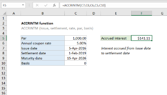
In finance, bonds prices are quoted "clean". The "clean price" of a bond excludes any interest accrued since the issue date or most recent coupon payment. The "dirty price" of a bond is the price including accrued interest. The ACCRINT function can be used to calculate accrued interest for a security that pays periodic interest, but pay attention to date configuration.
Date configuration
By default, ACCRINT will calculate accrued interest from the issue date. If the settlement date is in the first period, this works. However, if the settlement date is not in the first period, you probably don't want total accrued interest from the issue date but rather accrued interest from the last interest date (previous coupon date). As a workaround, based on the article here:
- set issue date to the previous coupon date
- set first_interest date to the previous coupon date
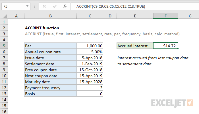
Note: According to Microsoft documentation, calc_method controls how total accrued interest is calculated when the date of settlement > first_interest. The default is TRUE, which returns the total accrued interest from issue date to settlement date. Setting calculation method to FALSE is supposed to return accrued interest from first_interest to settlement date. However, I was unable to produce this behavior. In the example below, issue date and first_interest date are set to the previous coupon date (as described above).
Example
In the example shown, we want to calculate accrued interest for a bond with a 5% coupon rate. The issue date is 5-Apr-2018, the settlement date is 1-Feb-2019, and the last coupon date is 15-Oct-2018. We want accrued interest from October 15, 2018 to February 1, 2019. The formula in F5 is:
=ACCRINT(C9,C9,C8,C6,C5,C12,C13,TRUE)
With these inputs, the ACCRINT function returns $14.72, with currency number format applied.
Entering dates
In Excel, dates are serial numbers. Generally, the best way to enter valid dates is to use cell references, as shown in the example. To enter valid dates directly inside a function, you can use the DATE function. To illustrate, the formula below has all values hardcoded. The DATE function is used to supply each of the three required dates:
=ACCRINT(DATE(2018,10,15),DATE(2018,10,15),DATE(2019,2,1),0.05,1000,2,0,TRUE)
Basis
The basis argument controls how days are counted. The ACCRINT function allows 5 options (0-4) and defaults to zero, which specifies US 30/360 basis. This article on wikipedia provides a detailed explanation of available conventions.
| Basis | Day count |
|---|---|
| 0 or omitted | US (NASD) 30/360 |
| 1 | Actual/actual |
| 2 | Actual/360 |
| 3 | Actual/365 |
| 4 | European 30/360 |
Notes
- In Excel, dates are serial numbers.
- All dates, plus frequency and basis, are truncated to integers.
- If dates are invalid (i.e. not actually dates) ACCRINT returns #VALUE!
- ACCRINT returns #NUM when:
- issue date >= settlement date
- rate < 0 or par <= 0
- frequency is not 1, 2, or 4
- Basis is out-of-range