Summary
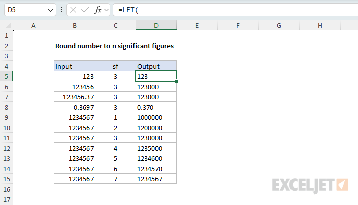
To round a number to s given number of significant figures (sometimes called significant digits), you can use a formula based on the LET, ROUND, LOG10, and TEXT functions. In the example shown, the formula in D5 is:
=LET(
    number,B5,
    sf,C5,
    dp,sf-(1+INT(LOG10(ABS(number)))),
    rounded,ROUND(number,dp),
    IF(dp>0,TEXT(rounded,"0."&REPT("0",dp)),TEXT(rounded,"0")))
This formula correctly handles decimal numbers with trailing zeros. If you don't need to handle decimal values with significant trailing zeros and always want a numeric result, see the simpler formula below.
Generic formula
=ROUND(number,digits-(1+INT(LOG10(ABS(number)))))
Explanation
In this example, the goal is to round a number to a given number of significant figures while preserving trailing zeros when needed. This is a tricky problem because Excel's rounding functions return numbers, and numbers don't preserve trailing zeros.
This article uses "significant figures" and "significant digits" interchangeably.
Table of contents
- What are significant figures?
- How significant figures work
- The challenge in Excel
- Formula structure
- Calculating decimal places (dp)
- Adjusting decimal places for ROUND
- Formatting the result
- Simple formula with numeric result
What are significant figures?
Significant figures (or significant digits) represent the meaningful digits in a number — the digits that carry real information about its precision. When you round to a given number of significant figures, you express a value with a specific level of accuracy, regardless of its magnitude. This matters because not all digits in a number are equally trustworthy. A scientist measuring a sample weight might record 0.003702 grams, but if the scale is only accurate to three significant figures, reporting all those digits implies false precision. The honest value is 0.00370 — three digits that actually mean something. Significant figures are often used in scientific notation to express the precision of a number.
How significant figures work
Significant figures count from the first non-zero digit, regardless of where the decimal point falls. Leading zeros are placeholders, not significant digits. Here are a few examples of rounding to 3 significant figures:
| Original | Rounded | Notes |
|---|---|---|
| 12345 | 12300 | First three digits kept |
| 3.697 | 3.70 | Trailing zero is significant |
| 0.3697 | 0.370 | Leading zero is not significant |
| 0.003697 | 0.00370 | Leading zeros are placeholders |
| 9876 | 9880 | Third digit rounds up |
Notice that the number of decimal places varies. What stays constant is the count of meaningful digits.
The challenge in Excel
Rounding to significant figures is straightforward in principle, but Excel makes it tricky. The core issue is that Excel's ROUND function returns a number, and numbers don't preserve trailing zeros. When you round 0.3697 to three significant figures, you end up with 0.37, which is mathematically correct, but displays in Excel as two significant figures.
This happens because trailing zeros after a decimal point have no effect on a number's value. To Excel, 0.37 and 0.370 are identical. The only way to force Excel to display trailing zeros is to return text instead of a number, which is why this formula uses TEXT function to format the final result.
Formula structure
In the example shown, the formula in D5 is:
=LET(
    number,B5,
    sf,C5,
    dp,sf-(1+INT(LOG10(ABS(number)))),
    rounded,ROUND(number,dp),
    IF(dp>0,TEXT(rounded,"0."&REPT("0",dp)),TEXT(rounded,"0")))
Let's break down the formula step-by-step.
The formula uses the LET function to define named variables that make the logic easier to follow:
numberis the number to round (B5)sfis the number of significant figures (C5)dpis the calculated decimal places neededroundedis the result of the ROUND function
Ultimately, dp is used to round the number to the correct number of decimal places like this:
=ROUND(number,dp) // actual rounding formula
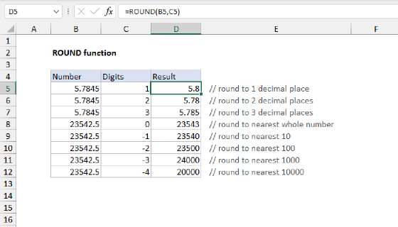
Calculating dp correctly is the crux of the problem. We need a number to give to the ROUND function that will preserve the requested number of significant figures, taking into account the magnitude of the number. Remember with ROUND that a negative number of digits works on the left side of the decimal. If we round 1234567 to an increasing number of significant digits, we would have:
=ROUND(1234567,-6) = 1000000 // 1 sig. digit
=ROUND(1234567,-5) = 1200000 // 2 sig. digits
=ROUND(1234567,-4) = 1230000 // 3 sig. digits
=ROUND(1234567,-3) = 1235000 // 4 sig. digits
Calculating decimal places (dp)
The challenge is how to calculate -6, -5, -4, and so on, depending on the number we are rounding. This calculation is handled by the snippet below:
sf-(1+INT(LOG10(ABS(number))))
Working from the inside out, we use the ABS function to ensure the formula works with negative numbers, since LOG10 only accepts positive values:
ABS(number) // absolute value of number
Then we use the LOG10 function to get the exponent of the number:
LOG10(ABS(number)) // exponent of number
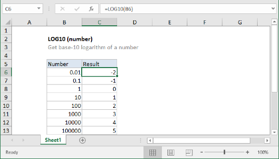
The LOG10 function returns the base 10 logarithm of a number:
=LOG10(10000) // returns 4
=LOG10(1000) // returns 3
=LOG10(100) // returns 2
=LOG10(10) // returns 1
=LOG10(1) // returns 0
=LOG10(0.1) // returns -1
=LOG10(0.01) // returns -2
=LOG10(0.001) // returns -3
=LOG10(0.0001) // returns -4
LOG10 tells us the power to which 10 must be raised to get the number. That is the exponent of 10. In other words, it tells us the magnitude of the number, which is related to the position of the first significant digit. Because it is the integer part of the result that we are interested in, we use the INT function to remove the decimal part:
- For 1234567 → INT(LOG10(1234567)) = 6 → first digit is in the millions place
- For 0.3697 → INT(LOG10(0.3697)) = -1 → first digit is in the tenths place
- For 0.003697 → INT(LOG10(0.003697)) = -3 → first digit is in the thousandths place
Adjusting decimal places for ROUND
Finally, we add 1 and subtract the result from the number of significant figures to get the decimal places needed:
sf-(1+INT(LOG10(ABS(number))))
The +1 adjustment accounts for the difference between how we count significant figures (starting from 1) and how the exponent represents position (starting from 0). For example, to round 1234567 to 1 significant figure, we need ROUND(1234567, -6). The exponent is 6, and we want 1 significant figure. The calculation 1 - (1+6) = -6 gives us exactly what we need. Without the +1, we'd get 1 - 6 = -5, which would incorrectly round to 1200000 instead of 1000000.
With the exponent in hand, the formula calculates the decimal places needed. Remember that ROUND accepts negative values for rounding to the left of the decimal point:
| Number | sf | Exponent | dp = sf-(1+exp) | Result |
|---|---|---|---|---|
| 1234567 | 3 | 6 | 3-(1+6) = -4 | 1230000 |
| 1234567 | 5 | 6 | 5-(1+6) = -2 | 1234600 |
| 0.3697 | 3 | -1 | 3-(1+(-1)) = 3 | 0.370 |
| 0.003697 | 3 | -3 | 3-(1+(-3)) = 5 | 0.00370 |
Formatting the result
The final piece handles the trailing zeros problem mentioned earlier:
IF(dp>0,TEXT(rounded,"0."&REPT("0",dp)),TEXT(rounded,"0"))
When dp is positive (meaning we need decimal places), the formula builds a format string dynamically using the TEXT function:
TEXT(rounded,"0."&REPT("0",dp))
The REPT function repeats a string a given number of times. In this case, it repeats the "0" string dp times. For example, for 0.3697 rounded to 3 significant figures, dp = 3, so the format becomes "0.000" which produces "0.370" with the trailing zero preserved:
=TEXT(0.370,"0."&REPT("0",3))
=TEXT(0.370,"0.000") // returns "0.370"
If dp is zero or negative (large numbers), no decimal places are needed, so the formula uses a simple "0" format. For example, for 1234567 rounded to 1 significant figure, dp = -6, so the format becomes "0" which produces "1000000":
=TEXT(1000000,"0") // returns "1000000"
Simple formula with numeric result
Because the formula above uses the TEXT function to return a final result, the result is text, not a number. This is unavoidable if you want trailing zeros displayed. It's fundamentally a formatting issue in Excel rather than a calculation issue. If you need a numeric result for further calculations and don't care about trailing zeros, you can use a simpler formula based on the ROUND function:
=ROUND(B5,C5-(1+INT(LOG10(ABS(B5)))))
This formula returns a true number rounded to the given number of significant figures, but it won't preserve trailing zeros like 0.370. This same code appears inside the more complicated LET version of the formula above and is explained in detail above.
Another option is to allow the LET function to return a result to the worksheet in a cell and use the VALUE function to convert the text result to a number in a separate formula if needed.