Summary
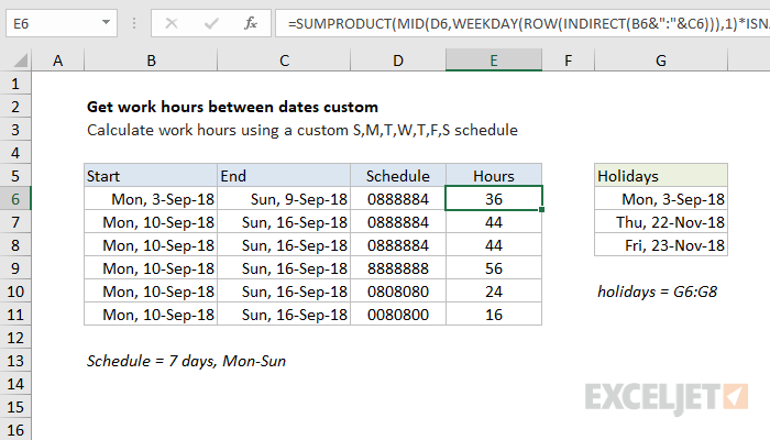
To calculate work hours between two dates with a custom schedule, you can use a formula based on the WEEKDAY and SUMPRODUCT functions, with help from ROW, INDIRECT, and MID. In the example shown, the formula in F8 is:
=SUMPRODUCT(MID(D6,WEEKDAY(ROW(INDIRECT(B6&":"&C6))),1)*ISNA(MATCH(ROW(INDIRECT(B6&":"&C6)),holidays,0)))
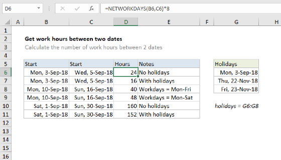
Which returns 36 hours, based on a custom schedule where 8 hours are worked Mon-Fri, 4 hours are worked on Saturday, and Monday September 3 is a holiday. Holidays are supplied as the named range G6:G8. The work schedule is entered as a text string in column D and can be changed as desired.
Note: This is an array formula that must be entered with Control + Shift + Enter. If you have a standard 8 hour workday, this formula is simpler.
Generic formula
=SUMPRODUCT(MID(schedule,WEEKDAY(ROW(INDIRECT(start&":"&end))),1)*ISNA(MATCH(ROW(INDIRECT(start&":"&end)),holidays,0)))
Explanation
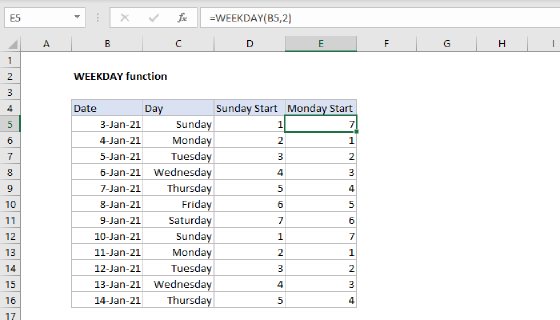
At the core, this formula uses the WEEKDAY function to figure out the day of week (i.e. Monday, Tuesday, etc.) for every day between the two given dates. WEEKDAY returns a number between 1 and 7. With default settings, Sunday=1 and Saturday = 7.
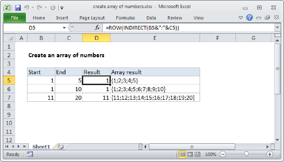
The trick to this formula is assembling an array of dates that you can feed into the WEEKDAY function. This is done with ROW with INDIRECT:
ROW(INDIRECT(B6&":"&C6))
ROW interprets the concatenated dates as row numbers and returns an array like this:
{43346;43347;43348;43349;43350;43351;43352}
Each number in the array represents a date. The WEEKDAY function then evaluates the array and returns an array of weekday values:
{2;3;4;5;6;7;1}
These numbers correspond to the day of week of each date. They are provided to the MID function as the start number argument, along with the value in D6, "0888884" for text:
MID("0888884",{2;3;4;5;6;7;1},1)
Because we are giving MID an array of start numbers, it returns an array of results like this:
{"8";"8";"8";"8";"8";"4";"0"}
These values correspond to the hours worked on each day from the start date to the end date. Note the values in this array are text, not numbers. To convert to actual numbers, we multiply by a second array created to manage holidays, as explained below. The math operation coerces the text to numeric values.
Holidays
To handle holidays, we use ISNA, MATCH, and the named range "holidays" like this:
ISNA(MATCH(ROW(INDIRECT(B6&":"&C6)),holidays,0))
This expression uses MATCH to locate dates that are in the named range holidays using the same array of dates generated above with INDIRECT and ROW. MATCH returns a number when holidays are found and the #N/A error when not. The ISNA function "flips" the results so that TRUE represents holidays and FALSE represents non-holidays. ISNA returns an array or results like this:
{FALSE;TRUE;TRUE;TRUE;TRUE;TRUE;TRUE}
Finally, both arrays are multiplied by each other inside SUMPRODUCT. The math operation coerces TRUE and FALSE to 1 and zero, and the text values in the first array to numeric values (as explained above), so in the end we have:
=SUMPRODUCT({8;8;8;8;8;4;0}*{0;1;1;1;1;1;1})
After multiplication, we have a single array inside SUMPRODUCT containing all working hours in the date range:
=SUMPRODUCT({0;8;8;8;8;4;0})
SUMPRODUCT then sums all items in the array and returns a result of 36.