Summary
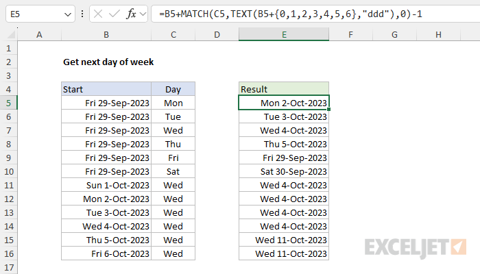
To get the next specified weekday (i.e. the next Monday, the next Tuesday, the next Wednesday, etc.) starting from a given start date, you can use a formula based on the MATCH function and the TEXT function. In the example shown, the formula in E5 is:
=B5+MATCH(C5,TEXT(B5+{0,1,2,3,4,5,6},"ddd"),0)-1
Where B5 contains a start date, and C5 contains the target weekday, given as the 3-letter abbreviation "Mon". The result is Monday, October 2, 2023 — the first Monday after Friday, September 29, 2023.
Generic formula
=A1+MATCH("Mon",TEXT(A1+{0,1,2,3,4,5,6},"ddd"),0)-1
Explanation
In this example, the goal is to get the next specified weekday, starting on a given start date. So for example, with a valid start date in column B, we want to be able to ask for the next Monday, the next Tuesday, the next Wednesday, and so on. This article describes two different ways of solving this problem. The first way, which appears in the worksheet shown above, is based on the TEXT function and the MATCH function. This method is flexible and intuitive since you can simply ask for the desired day of the week by name. The second method is based on the WEEKDAY function. This is the "traditional approach", although I find it harder to understand. Both approaches are explained below, and both work equally well.
I've now added a third option to solve this problem with the WORKDAY.INTL function below. This last approach is the simplest option, but it does involve using some cryptic custom codes. Also, note that the first two options will return the start date if it is already the target day of the week. The last option will always advance to the next target day of the week, even if the start date is already the target day of the week.
MATCH + TEXT option
One way to solve this problem is with the MATCH function and the TEXT function using a generic formula like this:
=A1+MATCH("Mon",TEXT(A1+{0,1,2,3,4,5,6},"ddd"),0)-1
In this formula, we assume the start date is in cell A1, and that our target day of the week is Monday, abbreviated "Mon". Here's how this formula works, working from the inside out:
- A1+{0,1,2,3,4,5,6}: This creates an array of dates that includes the start date plus the next six days.
- TEXT(A1+{0,1,2,3,4,5,6},"ddd"): This converts each date in the array to a text string representing the abbreviated day of the week (e.g., "Sun", "Mon", "Tue", etc.).
- MATCH("Mon",TEXT(A1+{0,1,2,3,4,5,6},"ddd"),0): This searches for the position of the specified day ("Mon" for Monday) in the array of abbreviated day names. The position becomes the number of days to add to the original date in A1 to reach the next specified weekday.
- -1: Since the array includes the current day, we subtract 1 to adjust the position to the correct number of days to add.
- A1 + : Finally, the number of days calculated above is added to the original date in A1 to get the date of the next specified weekday.
The main trick in this formula is this: TEXT(A1+{0,1,2,3,4,5,6},"ddd"). Excel evaluates this part of the formula in E5 as follows:
=TEXT(B5+{0,1,2,3,4,5,6},"ddd")
=TEXT(45198+{0,1,2,3,4,5,6},"ddd")
=TEXT({45198,45199,45200,45201,45202,45203,45204},"ddd")
={"Fri","Sat","Sun","Mon","Tue","Wed","Thu"}
What we see above is that the date in cell B5 (September 29, 2023) is serial number 45198 in Excel's date system. When we add the array constant {0,1,2,3,4,5,6} to this number, we get an array that represents Sep. 29 plus the next 6 days. The text string "ddd" is a custom number format for a 3-letter abbreviation for weekday names. TEXT runs on all seven dates and returns their abbreviated names in an array like this:
{"Fri","Sat","Sun","Mon","Tue","Wed","Thu"}
When we drop this array back into the original formula, we get the following:
=B5+MATCH(C5,{"Fri","Sat","Sun","Mon","Tue","Wed","Thu"},0)-1
=B5+MATCH("Mon",{"Fri","Sat","Sun","Mon","Tue","Wed","Thu"},0)-1
=B5+4-1
=45198+4-1
=45201
With "Mon" in cell C5, MATCH returns 4, and the final result is 45201, which is Monday, October 2, 2023.
This formula is intuitive and flexible since you can easily change the target day by replacing "Mon" with the abbreviation of another day of the week. It will return the original date in A1 if it is already the specified weekday, and the next occurrence of the specified weekday otherwise. There is no need to know the numeric values for each day, as with the WEEKDAY formula below.
WEEKDAY option
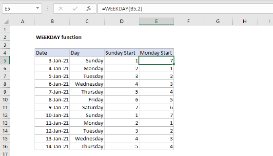
Another more traditional way to solve this problem is with the WEEKDAY function. The WEEKDAY function takes a date and returns a number between 1-7 representing the day of the week. By default, WEEKDAY uses a scheme where Sunday =1, Monday=2, Tuesday=3, Wednesday=4, Thursday=5, Friday=6, and Saturday=7. So, for example, WEEKDAY returns 6 for September 29, 2023, which is a Friday:
=WEEKDAY("29-Sep-2023") // returns 6
We can use this behavior to create a formula that returns the next given weekday with a generic formula like this:
=A1+7-WEEKDAY(A1+7-n)
Where A1 contains the start date, and n represents the day number of the weekday you want. So for example, in the first formula below n is 7 to get the next Saturday while in the second formula n is 2 to get the next Monday:
=A1+7-WEEKDAY(A1+7-7) // next Saturday
=A1+7-WEEKDAY(A1+7-2) // next Monday
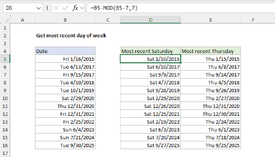
You can see this approach used in the worksheet below, where start dates appear in column B, and the target weekday is specified with a day number in column C:
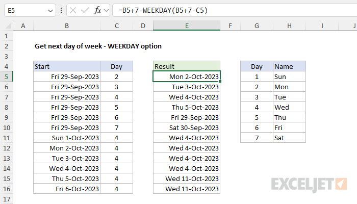
Notes: (1) The table in G5:H11 is a key for day numbers, provided for reference only. (2) When the given date is already the desired day of week, the original date is returned.
This formula is more difficult to understand than the first formula. The gist is that it first rolls the date forward by 7 days, then steps back to the correct date by subtracting the result of a calculation that uses the WEEKDAY function. Working from the inside out, here are the steps
- A1 + 7: Moves forward 7 days to the same weekday of the next week.
- A1 + 7 - n: Shifts back by n days to a "reference day". The result depends on the weekday provided as n.
- WEEKDAY(A1 + 7 - n): Calculates the weekday number of the reference day.
- A1 + 7 - WEEKDAY(A1 + 7 - n): Subtracts the weekday number of the reference day from the date calculated in step 1.
The key is the reference day calculated by A1 + 7 - n. This reference day is always in the same week as the original date A1. By calculating the WEEKDAY of the reference day and subtracting it from A1 + 7, we are essentially finding the next occurrence of the desired weekday in the current week. For example, assume A1 contains the date Sep 29, 2023 (which is a Friday), and n is given as 2 (for Monday):
- A1 + 7: Sep 29, 2023 + 7 days = Oct 6, 2023 (a Friday).
- A1 + 7 - n: Oct 6, 2023 - 2 (since n is 2 for Monday) = Oct 4, 2023 (a Wednesday).
- WEEKDAY(A1 + 7 - n): WEEKDAY(Oct 4, 2023) = 4 (Wednesday is 4 in the default scheme).
- A1 + 7 - WEEKDAY(A1 + 7 - n): Oct 6, 2023 - 4 = Oct 2, 2023 (a Monday).
The final result is Oct 2, 2023, the next Monday after the given date.
Next day of week from today
To get the next day of week starting with the current date, you can use the TODAY function in place of a date in A1 like so:
=TODAY()+7-WEEKDAY(TODAY()+7-n)
WORKDAY.INTL option
Many months after I wrote the article above, I ran into another way to solve this problem with the WORKDAY.INTL function and a generic formula like this:
=WORKDAY.INTL(start_date, 1, "custom_code")
WORKDAY.INTL calculates the "next" working day n days in the past or future, taking into non-working days and (optionally) holidays. In the formula above, start_date is the date to start from, and 1 is days - the number of days to move forward. The tricky part is the "custom_code" provided for the weekend argument, which involves "hacking" a hidden feature of WORKDAY.INTL.
The third argument in WORKDAY.INTL is weekend, which specifies which days of the week should be treated as weekends. Normally provided as a numeric code, weekday can also be provided as a 7-digit binary code that covers all seven days of the week, Monday through Saturday. In this scheme, a 1 indicates a weekend (non-working) day, and a 0 indicates a workday. For example, to get the next regular workday Monday through Friday, you can use the code "0000011" like this:
=WORKDAY.INTL(A1,1,"0000011") // next workday, Mon-Fri
Note: Zeros are "workdays" and the 1s are "weekends".
By carefully creating a code that only allows one day of the week, we can hijack this feature and use the WORKDAY.INTL function to find the next target day of the week like this:
=WORKDAY.INTL(A1,1,"0111111") // next Monday
=WORKDAY.INTL(A1,1,"1011111") // next Tuesday
=WORKDAY.INTL(A1,1,"1101111") // next Wednesday
=WORKDAY.INTL(A1,1,"1110111") // next Thursday
=WORKDAY.INTL(A1,1,"1111011") // next Friday
=WORKDAY.INTL(A1,1,"1111101") // next Saturday
=WORKDAY.INTL(A1,1,"1111110") // next Sunday
This formula is simpler than either of the two formulas above, but there is one key difference: it will always advance to the next target day of week, even if the start date is already the target day of the week.