Summary
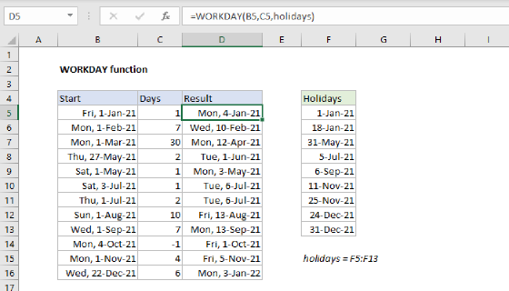
To add or subtract business days (workdays) to a date, you can use a formula based on the WORKDAY function. In the example, the formulas in G5 and G6 are:
=WORKDAY(start,days)
=WORKDAY(start,days,holidays)
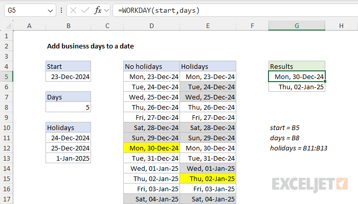
Where start (B5), days (B8), and holidays (B11:B13) are named ranges. Both formulas show the result of adding 5 workdays, starting from December 23, 2024. The first formula excludes weekends only returns December 30, 2024. The second formula excludes weekends and holidays and returns January 2, 2025.
Notes: This is a basic example based on a standard 5-day workweek. If you need to customize which days are workdays and non-work days, see this page. (2) The dates in columns D and E are not required in this solution, they exist only to help visualize how the WORKDAY function evaluates working and non-working days and arrives at a final result. See below for details on how this is set up.
Generic formula
=WORKDAY(start,days,holidays)
Explanation
In this example, the goal is to calculate a workday n days in the future while excluding weekends and optionally holidays. For convenience, start (B5), days (B8), and holidays (B11:B13) are named ranges. The dates in columns D and E are dynamically generated based on the start date in B5. Conditional formatting is used to shade excluded days in gray and to highlight the final calculated dates in yellow. All calculations are performed with the WORKDAY function.
The WORKDAY function
Excel's WORKDAY function takes a date and returns the next working day n days in the future or past. You can use the WORKDAY function to calculate ship dates, delivery dates, and completion dates that need to take into account working and non-working days. For example, with a start date in cell A1, you can calculate a date 5 workdays in the future with a formula like this:
=WORKDAY(A1,5)
In this basic configuration, WORKDAY will automatically exclude Saturdays and Sundays, and return the next workday 5 days after the starting date. WORKDAY can optionally exclude holidays as well as weekends. For example, with a list of holiday dates in the range C1:C3 you can calculate the next workday 5 days after the starting date in A1 while also excluding holidays:
=WORKDAY(A1,5,C1:C3)
WORKDAY solution
The worksheet in the example shown contains 3 named ranges: start (B5), days (B8), and holidays (B11:B13). The names are for convenience only and make the formulas easier to read. The formula in cell G5 calculates the next working day 5 days after December 23, 2024, and does not take into account holidays:
=WORKDAY(start,days) // returns 30-Dec-2024
The result is Monday, December 30, 2024. The formula in cell G6 performs the same calculation but also excludes the dates in holidays (B11:B13).
=WORKDAY(start,days,holidays) // returns 02-Jan-2025
The result is Thursday, January 2, 2025. Notice the holidays in the range B11:B13 are valid dates.
Data visualization
The dates in columns D and E are not required in this solution, they exist only to help visualize how the WORKDAY function evaluates working and non-working days and arrives at a final result. The dates are dynamically generated based on the start date with SEQUENCE function. The formula in D5 and E5 is the same and looks like this:
=SEQUENCE(13,1,start)
- rows - 13 (arbitrary, can be increased or decreased)
- columns - 1
- start - start (cell B5, which contains 23-Dec-2024)
With this configuration, SEQUENCE generates 13 dates, starting with the start date in cell B5. This works because Excel dates are stored as serial numbers. To make it easy to see what day of the week each date is, the dates in the range D5:E17 are formatted with the following custom number format:
ddd, dd-mmm-yy
This date format displays an abbreviated day name (e.g. "Mon") followed by the date.
Shading non-working days with conditional formatting
The gray shading indicates which days are not workdays and this formatting is applied with conditional formatting. The key is to use the WORKDAY function to trigger the formatting to accurately illustrate how WORKDAY evaluates working and non-working days in this date range. In column D the conditional formatting is triggered by this formula:
=WORKDAY(D5-1,1)<>D5
Essentially, we are asking WORKDAY if each date is not a workday by running the date through the workday function and then checking if the date is not equal to itself. Because WORKDAY will not evaluate a date if zero is provided for days, we use a workaround formula that first subtracts 1 day from the start date and then asks for the next workday. If the result from WORKDAY is not equal to the original date, it means WORKDAY shifted the date because it is a non-working day. The formula returns TRUE and the shading is applied.
To shade non-working days in column E, we use this formula:
=WORKDAY(E5-1,1,holidays)<>E5
The two formulas are very similar, but this formula also provides the named range holidays (B11:B13). The result is that more days are shaded since both weekends and holidays are non-working days.
Highlighting final results with conditional formatting
The formulas that highlight the final calculated dates in yellow look like this:
=D5=$G$5 // column D
=E5=$G$6 // column E
In column D, the first formula checks for a date equal to the result in G5. In column E, the second formula checks for a date equal to the result in cell G6. Because G5 and G6 are not defined as named ranges, we must use the absolute references $G$5 and $G$6. To create independent conditional formatting rules that do not require the dates in column G, you can use the WORKDAY function directly in formulas like this:
=D5=WORKDAY(start,days)
=E5=WORKDAY(start,days,holidays)
The result is the same. The difference is that the conditional formatting is unlinked from column G results and therefore self-contained.
Conditional formatting summary
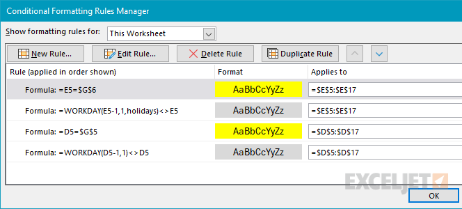
In total, there are four conditional formatting rules used in the workbook shown as seen below:
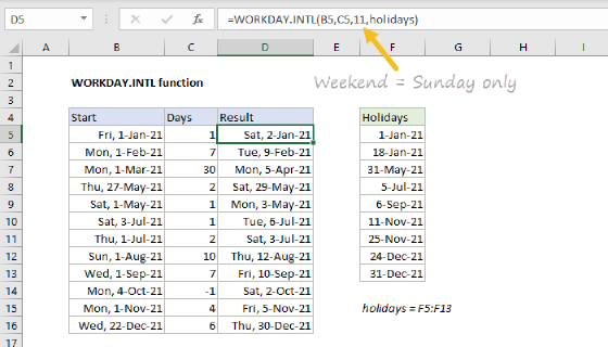
If you need to implement a custom work schedule (i.e. a 4-day workweek, a 6-day workweek, etc.) you will want to switch to the WORKDAY.INTL function which provides more flexibility. See this example for details.