Summary
To use XLOOKUP to find an exact match, you'll need to supply a lookup value, a lookup range, and a result range. In the example shown, the formula in H6 is:
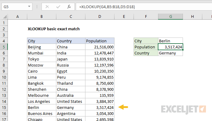
=XLOOKUP(G4,B5:B18,D5:D18)
which returns 3,517,424, the population for Berlin from column D.
Generic formula
=XLOOKUP(value,rng1,rng2)
Explanation
In the example shown, cell G4 contains the lookup value, "Berlin". XLOOKUP is configured to find this value in the table, and return the population. The formula in G5 is:
=XLOOKUP(G4,B5:B18,D5:D18) // get population
- The lookup_value comes from cell G4
- The lookup_array is the range B5:B18, which contains City names
- The return_array is D5:D18, which contains Population
- The match_mode is not provided and defaults to 0 (exact match)
- The search_mode is not provided and defaults to 1 (first to last)
To return County instead of population, only the return array is changed. The formula in G6 is:
=XLOOKUP(G4,B5:B18,C5:C18) // get country
XLOOKUP vs VLOOKUP
The equivalent VLOOKUP formula to retrieve population is:
=VLOOKUP(G4,B5:D18,3,0)
There are a few notable differences which make XLOOKUP more flexible and predictable:
- VLOOKUP requires the full table array as the second argument. XLOOKUP requires only the range with lookup values.
- VLOOKUP requires a column index argument to specify a result column. XLOOKUP requires a range.
- VLOOKUP performs an approximate match by default. This behavior can cause serious problems. XLOOKUP performs an exact match by default.
Dynamic Array Formulas are available in Office 365 only.