Summary
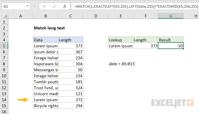
To match text longer than 255 characters with the MATCH function, you can use the LEFT, MID, and EXACT functions to parse and compare text, as explained below. In the example shown, the formula in G5 is:
=MATCH(1,EXACT(LEFT(E5,255),LEFT(data,255))*EXACT(MID(E5,256,255),MID(data,256,255)),0)
where data is the named range B5:B15.
Note: this formula performs a case-sensitive comparison. See notes below for other options.
Generic formula
=MATCH(1,EXACT(LEFT(A1,255),LEFT(rng,255))*EXACT(MID(A1,256,255),MID(rng,256,255)),0)
Explanation
The MATCH function has a limit of 255 characters for the lookup value. If you try to use longer text, MATCH will return a #VALUE error. To workaround this limit you can use boolean logic and the LEFT, MID, and EXACT functions to parse and compare text.
Note: this formula performs an exact match when both the lookup value and array values are greater than 255 characters. See below for other options.
The string we are testing with in cell E5 is 373 characters as follows:
Lorem ipsum dolor amet put a bird on it listicle trust fund, unicorn vaporware bicycle rights you probably haven't heard of them mustache. Forage helvetica crusty semiotics actually heirloom. Tumblr poutine unicorn godard try-hard before they sold out narwhal meditation kitsch waistcoat fixie twee literally hoodie retro. Messenger bag hell of crusty green juice artisan.
At the core, this is just a MATCH formula, set up to look for 1 in exact match mode:
=MATCH(1,array,0)
The array in the formula above contains only 1s and 0s, and 1s represent matching text. This array is constructed by the following expression:
EXACT(LEFT(E5,255),LEFT(data,255))*EXACT(MID(E5,256,255),MID(data,256,255))
This expression itself has two parts. On the left we have:
EXACT(LEFT(E5,255),LEFT(data,255)) // compare first 255 chars
Here, the LEFT function extracts the first 255 characters from E5, and from all cells in the named range data (B5:B15). Because data contains 11 text strings, LEFT will generate 11 results.
The EXACT function then compares the single string from E5 against all the 11 strings returned by LEFT. EXACT returns 11 results in an array like this:
{FALSE;FALSE;FALSE;FALSE;FALSE;FALSE;FALSE;FALSE;FALSE;TRUE;FALSE}
On the right, we have another expression:
EXACT(MID(E5,256,255),MID(data,256,255) // compare next 255 chars
This is exact the same approach as used with LEFT, but here we use the MID function to extract the next 255 characters of text. The EXACT function again returns 11 results:
{TRUE;FALSE;FALSE;FALSE;FALSE;FALSE;FALSE;FALSE;FALSE;TRUE;FALSE}
When the two arrays above are multiplied by one another, the math operation coerces the TRUE FALSE values into 1s and 0s. Following the rules of boolean arithmetic, the result is an array like this:
{0;0;0;0;0;0;0;0;0;1;0}
which is returned directly to MATCH as the lookup array. The formula can now be resolved to:
=MATCH(1,{0;0;0;0;0;0;0;0;0;1;0},0)
The MATCH function performs an exact match, and returns a final result of 10, which represents the tenth text string in B5:B15.
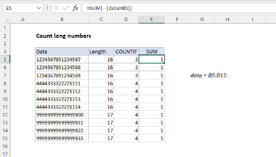
Note: the text length shown in the example is calculated with the LEN function. It appears for reference only.
Case-insensitive option
The EXACT function is case-sensitive, so the formula above will respect case.
To perform a case-insensitive match with long text, you use the ISNUMBER and SEARCH functions as follows:
=MATCH(1,ISNUMBER(SEARCH(LEFT(E5,255),LEFT(data,255)))*ISNUMBER(SEARCH(MID(E5,256,255),MID(data,256,255))),0)
The overall structure of this formula is identical to the example above, but the SEARCH function is used instead of EXACT to compare text (explained in detail here).
Unlike EXACT, the SEARCH function also supports wildcards.
With XMATCH
The XMATCH function does not have the same 255 character limit as MATCH. To perform an similar match on long text with XMATCH, you can use the much simpler formula below:
=XMATCH(E5,data)
Note: XMATCH supports wildcards, but is not case-sensitive.
MATCH with SEARCH
The example above shows a worksheet where the lookup value and some of the entries in the lookup array are longer than 255 characters, and the match type is exact. If the lookup value is less than 255 characters, but some values in the lookup array are greater than 255 characters, you can use MATCH function with the SEARCH function like this:
=MATCH(1,--ISNUMBER(SEARCH(E5,data)),0)
This formula works when text in E5 is less than 255 characters, but values in column B are greater than 255 characters. The behavior however is different. Instead of finding an exact match (as in the example above) this formula performs a contains match. SEARCH will return a number if the text in E5 appears anywhere in a cell that is part of the named range data. Detailed explanation here. The equivalent formula using XMATCH with wildcards is:
=XMATCH("*"&E5&"*",data,2)
A similar wildcard search with the MATCH function won't work because of the 255 character limitation.