Summary
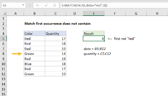
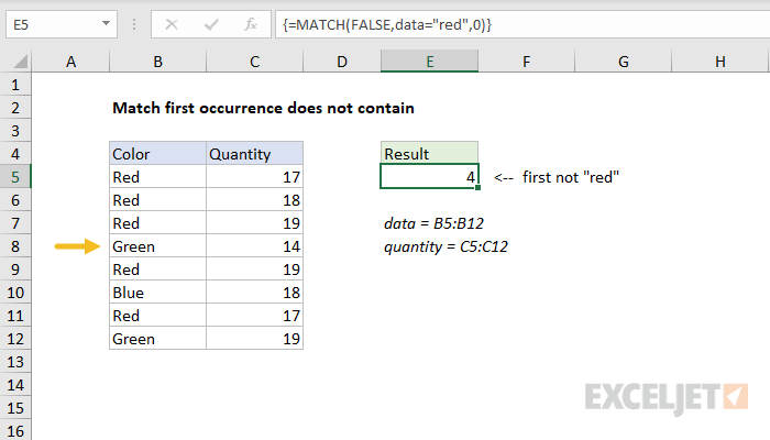
To get the position of the first match that does not contain a specific value, you can use an array formula based on the MATCH, SEARCH, and ISNUMBER functions. In the example shown, the formula in E5 is:
{=MATCH(FALSE,data="red",0)}
where "data" is the named range B5"B12.
Note: this is an array formula and must be entered with control + shift + enter, except in Excel 365.
Generic formula
{=MATCH(FALSE,logical_test,0)}
Explanation
This formula depends on a TRUE or FALSE result from a logical test, where FALSE represents the value you are looking for. In the example, the logical test is data="red", entered as the lookup_array argument in the MATCH function:
=MATCH(FALSE,data="red",0)
Once the test is run, it returns an array or TRUE and FALSE values:
=MATCH(FALSE,{TRUE;TRUE;TRUE;FALSE;TRUE;FALSE;TRUE;FALSE},0)
With the lookup_value set to FALSE, and match_type set to zero to force and exact match, the MATCH function returns 4, the position of the first FALSE in the array.
Get associated value
To retrieve the associated value from the Quantity column, where "quantity" is the named range C5:C12, you can use INDEX and MATCH together:
{=INDEX(quantity,MATCH(FALSE,data="red",0))}
Literal contains
If you need to match the first value that literally "does not contain", you can use a variant of the formula. For example to match the first value in data that does not contain an "r", you can use:
{=MATCH(FALSE,ISNUMBER(SEARCH("r",data)),0)}
Note: this is an array formula and must be entered with control + shift + enter, except in Excel 365.
For more details about ISNUMBER + SEARCH, see this page.