Summary
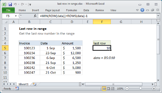
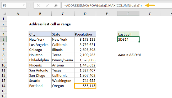
To get the last column in a range, you can use a formula based on the COLUMN and COLUMNS functions. In the example shown, the formula in cell F5 is:
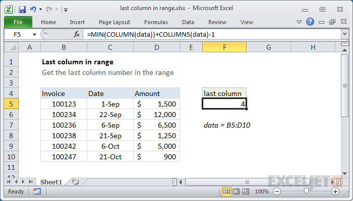
=MIN(COLUMN(data))+COLUMNS(data)-1
where data is the named range B5:D10.
Generic formula
=MIN(COLUMN(rng))+COLUMNS(rng)-1
Explanation
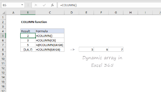
When given a single cell reference, the COLUMN function returns the column number for that reference. However, when given a range that contains multiple columns, the COLUMN function will return an array that contains all column numbers for the range.
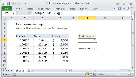
If you want only the first column number, you can use the MIN function to extract just the first column number, which will be the lowest number in the array:
=MIN(COLUMN(data)) // first column
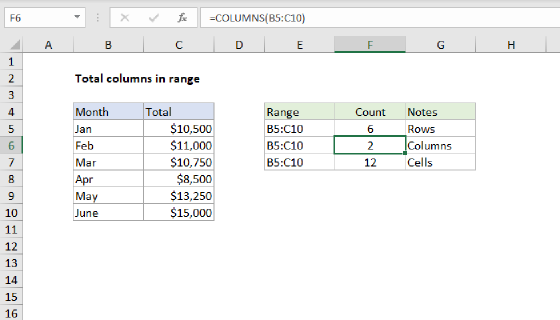
Once we have the first column, we can add the total columns in the range and subtract 1 to get the last column number.
Index version
Instead of MIN, you can also use INDEX to get the last row number:
=COLUMN(INDEX(data,1,1))+COLUMNS(data)-1
This is possibly a bit faster for large ranges, since INDEX just supplies a single cell to COLUMN.
Simple version
When a formula returns an array result, Excel will display the first item in the array if the formula is entered in a single cell. This means that in practice, you can sometimes use a simplified version of the formula:
=COLUMN(data)+COLUMNS(data)-1
But be aware that this will return an array for a multi-column range.
Inside formulas, it's sometimes necessary to make sure you are dealing with only one item, and not an array. In that case, you'll want to use the full version above.