Get relative column numbers in range

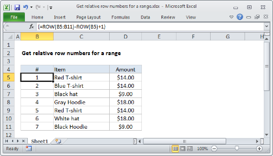
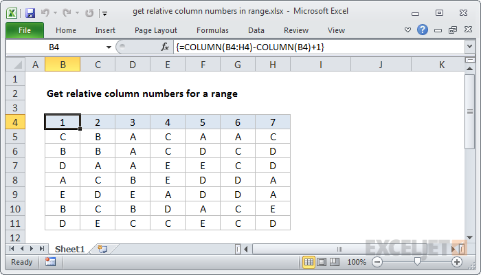
To get a full set of relative column numbers in a range, you can use an array formula based on the COLUMN function.

In the example shown, the array formula in B4:H4 is:

{=COLUMN(B4:H4)-COLUMN(B4)+1}

On the worksheet, this must be entered as multi-cell array formula using Control + Shift + Enter

This is a robust formula that will continue to generate relative numbers even when columns are inserted in front of the range.

How this formula works

The first COLUMN function generates an array of 7 numbers like this:

{2,3,4,5,6,7,8}

The second COLUMN function generates an array with just one item like this:

{2}

which is then subtracted from the first array to yield:

{0,1,2,3,4,5,6}

Finally, 1 is added to get:

{1,2,3,4,5,6,7}

With a named range

You can adapt this formula to use with a named range. For example, in the above example, if you created a named range "data" for B4:H4, you can use this formula to generate column numbers:

{=COLUMN(data)-COLUMN(INDEX(data,1,1))+1}

In other array formulas

You'll encounter this formula in other array formulas that need to process data column-by-column.