Get pivot table subtotal

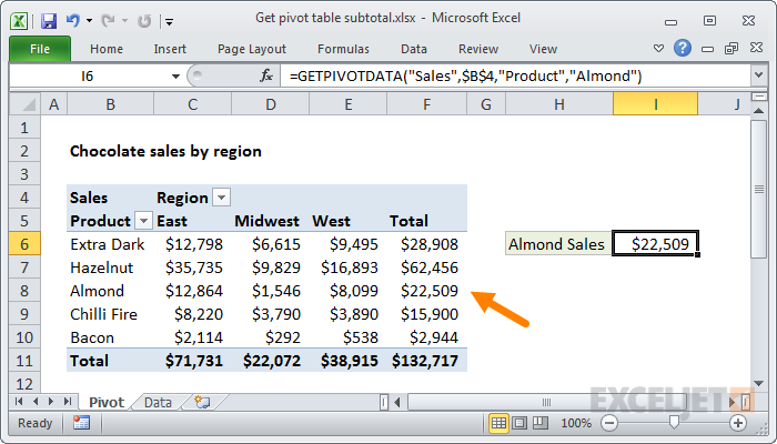
To get the subtotal for a value field in a pivot table, you can use the GETPIVOTDATA function. In the example shown, the formula in I6 is:

=GETPIVOTDATA("Sales",$B$4,"Product","Almond")

Although you can reference any cell in a pivot table with a normal reference (i.e. F8) the GETPIVOTDATA will continue to return correct values even when the pivot table changes.

Explanation

To use the GETPIVOTDATA function, the field you want to query must be a value field in the pivot table, subtotaled at the right level.

In this case, we want a subtotal of the "sales" field, so we provide the name the field in the first argument, and supply a reference to the pivot table in the second:

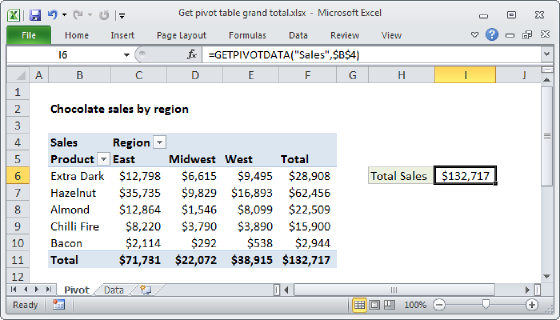
=GETPIVOTDATA("Sales",$B$4)

This will give us the grand total. The pivot_table reference can be any cell in the pivot table, but by convention we use the upper left cell.

To get the subtotal for the "Almond" product, we need to extend the formula as follows:

=GETPIVOTDATA("Sales",$B$4,"Product","Almond")

Additional pivot table fields are entered as field/item pairs, so we have now added the field "Product" and the item "Almond".

More specific subtotal

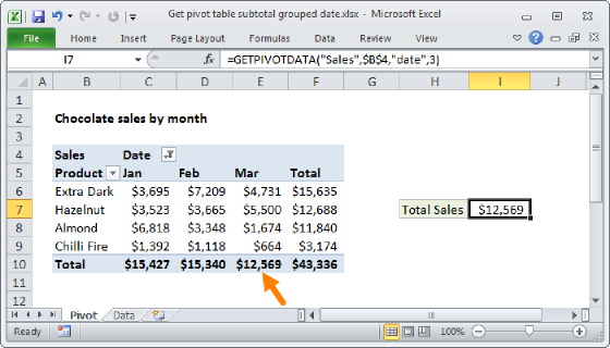
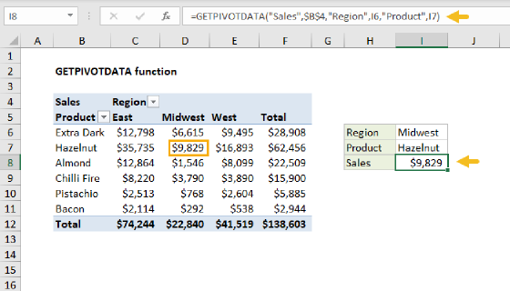
To get a more specific subtotal, like the "Almond" product in the "West" region, add an additional field/item pair:

=GETPIVOTDATA("Sales",$B$4,"Product","Almond","Region","West")

Note: GETPIVOTDATA will return a value field based on current "summarize by" settings (sum, count, average, etc.). This field must be visible in the pivot table.