Summary
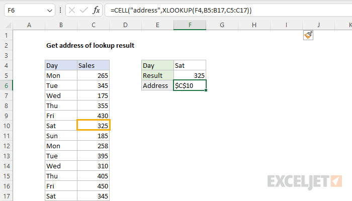
To get the address of the result returned by the XLOOKUP function or the INDEX function, you can use the CELL function. In the example shown, the formula in cell F6 is:
=CELL("address",XLOOKUP(F4,B5:B17,C5:C17))
The result is $C$10, the address of the cell returned by XLOOKUP. See below for an INDEX and MATCH example.
Note: the CELL function is a volatile function and can cause performance problems in large or complex worksheets. It is used in this example to show how to troubleshoot or confirm a lookup result.
Generic formula
=CELL("address",XLOOKUP(value,range,range))
Explanation
There are certain functions in Excel that return a cell reference as a result rather than a value. Two of these functions are XLOOKUP and INDEX. The presence of the cell reference in the result is not obvious, because Excel immediately resolves the reference to the value in that cell. You can check the reference returned by XLOOKUP or INDEX with the CELL function. This can be useful when debugging a lookup formula to confirm the result being returned.
XLOOKUP function
XLOOKUP is a function in Excel that returns a cell reference as a result instead of a value. You can inspect the reference returned by XLOOKUP by wrapping the formula in the CELL function with "address" as info_type. In the example shown, the formula in cell F6 is:
=CELL("address",XLOOKUP(F4,B5:B17,C5:C17))
Working from the inside out, the formula is an ordinary XLOOKUP formula:
=XLOOKUP(F4,B5:B17,C5:C17)
With a lookup value of "Sat" in cell F4, XLOOKUP returns 325, the Sales amount on the first entry for Saturday. However, underneath the surface, XLOOKUP is actually returning a reference to cell C10. We can check that result by nesting the XLOOKUP function inside the CELL function, and providing "address" for the info_type argument:
=CELL("address",XLOOKUP(F4,B5:B17,C5:C17)) // returns $C$10
The CELL function returns $C$10, the address of the cell returned by XLOOKUP. Note that if we configure XLOOKUP to perform a reverse search, by providing -1 for the search_mode argument, the result is $C$17:
=CELL("address",XLOOKUP(F4,B5:B17,C5:C17,,,-1)) // returns $C$17
This is the address of the second (and last) entry for Saturday in the data.
INDEX and MATCH
Like the XLOOKUP function, the INDEX function is another function that returns an address. The equivalent INDEX and MATCH formula that retrieves the Sales amount for "Sat" in F4 is:
=INDEX(C5:C17,MATCH(F4,B5:B17,0))
By wrapping the formula in the CELL function, we can get Excel to show us the address to the cell returned by INDEX:
=CELL("address",INDEX(C5:C17,MATCH(F4,B5:B17,0))) // returns $C$10
The CELL function returns $C$10, the address of the cell returned by INDEX.