Summary
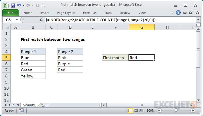
To retrieve the first match in two ranges of values, you can use a formula based on the INDEX, MATCH, and COUNTIF functions. In the example shown, the formula in G5 is:
=INDEX(range2,MATCH(TRUE,COUNTIF(range1,range2)>0,0))
where "range1" is the named range B5:B8, "range2" is the named range D5:D7.
Generic formula
=INDEX(range2,MATCH(TRUE,COUNTIF(range1,range2)>0,0))
Explanation
In this example the named range "range1" refers to cells B5:B8, and the named range "range2" refers to D5:D7. We are using named ranges for convenience and readability only; the formula works fine with regular cell references as well.
The core of this formula is INDEX and MATCH. The INDEX function retrieves a value from range2 that represents the first value in range2 that is found in range1. The INDEX function requires an index (row number) and we generate this value using the MATCH function, which is set to match the value TRUE in this portion of the formula:
MATCH(TRUE,COUNTIF(range1,range2)>0,0)
Here, the match value is TRUE, and the lookup array is created with COUNTIF here:
COUNTIF(range1,range2)>0
COUNTIF returns a count of the range2 values that appear in range1. Because range2 contains multiple values, COUNTIF will return multiple results that look like this:
{0;0;1}
We use ">0" to force all results to either TRUE or FALSE:
{FALSE;FALSE;TRUE}
Then MATCH does its thing and returns the position of the first TRUE (if any) that appears, in this case, the number 3.
Finally, INDEX returns the value at that position, "Red".