Summary
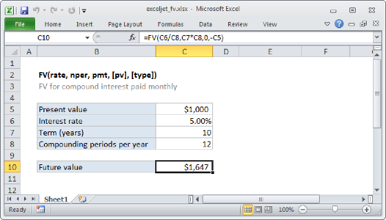
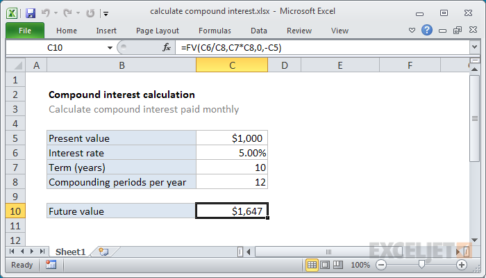
To calculate compound interest in Excel, you can use the FV function. This example assumes that $1000 is invested for 10 years at an annual interest rate of 5%, compounded monthly. In the example shown, the formula in C10 is:
=FV(C6/C8,C7*C8,0,-C5)
The FV function returns approximately 1647 as a final result.
Generic formula
=FV(rate,nper,pmt,pv)
Explanation
Compound interest is a financial concept that describes how an initial investment grows over time, taking into account not only the interest earned on the initial amount but also the interest earned on the interest itself. Compound interest allows your money to grow exponentially, which makes it a powerful tool for building wealth over the long term. To calculate the effect of compound interest in Excel, you can use the FV function, which is designed to calculate the future value of an investment.
FV function
The FV function, short for "Future Value," calculates the future value of an investment taking into account a constant interest rate and optional periodic payments. The FV function uses the following syntax:
=FV(rate,nper,pmt,[pv],[type])
Each argument has the following meaning:
- rate: The interest rate for each period.
- nper: The number of periods.
- pmt: The payment made each period (optional).
- pv: The present value or initial investment.
- [type]: Optional argument to indicate when payments are due.
To calculate compound interest in this example, we need to provide the FV function with the number of periods, the periodic payment, and the present value like this:
=FV(C6/C8,C7*C8,0,-C5)
- rate: C6/C8 (5%/12)
- nper: C7C8 (1012)
- pmt: 0 (no payment)
- pv: -C5 (-1000)
- [type]: Not needed
To get the rate (which is the period rate), we divide the annual rate (5%) by the compounding periods per year (12). To get the number of periods (nper), we multiply the term in years (10) by the periods per term (12). There is no periodic payment in this example, so we use zero for pmt. Finally, we provide the present value (pv) as -1000. By convention, the present value is input as a negative value because the initial investment of $1000 "leaves your wallet" and is transferred to the bank for the investment term. Putting it all together, Excel evaluates the formula like this:
=FV(C6/C8,C7*C8,0,-C5)
=FV(0.05/12,10*12,0,-1000)
=FV(0.00417,120,0,-1000)
=1647
The FV function returns approximately 1647 as a final result. This is the value of a $1,000 investment, compounded monthly with a 5% annual interest rate over 10 years.
For a more detailed example, see this page: Simple investing worksheet