Details
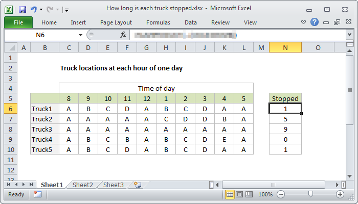
A couple weeks ago, a reader sent me an interesting question about tracking the "stopped time" for a fleet of trucks. The trucks are tracked by GPS so a location is recorded at each hour of the day for each truck. The data looks something like this:

The challenge: what formula in column N will correctly calculate total hours stopped?
I've simplified this a bit by replacing actual GPS coordinates with locations labeled A-E, but the concept remains the same.
The puzzle
For how many hours was each truck stopped?
Or, in Excel-speak:
What formula will calculate the total hours each truck was stopped?
For example, we know Truck1 was stopped for 1 hour because its location was recorded as "A" at both 4 PM and 5 PM.
Assumptions
- There are 5 locations with these names: A, B, C, D, E
- A truck at the same location for two consecutive hours = 1 hour stopped
Got a formula that will do it?
Download the workbook and share your formula in the comments below. As with so many things in Excel, there are many ways to solve this problem!
In this case, the versatile SUMPRODUCT is an elegant way to solve this problem:
=SUMPRODUCT(--(C6:K6=D6:L6))
Note ranges C6:K6 are offset by one column. In essence, we are comparing "previous positions" with "next positions", and counting cases where the previous position is the same as the next position.
For the data in row 6, the comparison operation creates an array of TRUE FALSE values:
{FALSE,FALSE,FALSE,FALSE,FALSE,FALSE,FALSE,FALSE,TRUE}
The double negative then coerces the TRUE FALSE values to ones and zeros, and SUMPRODUCT is simply the sum of the array, which is 1:
=SUMPRODUCT({0,0,0,0,0,0,0,0,1})


