Summary
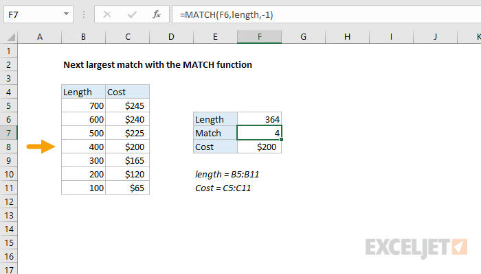
To look up the "next largest" match in a set of values, you can use the MATCH function in approximate match mode, with -1 for match type. In the example shown, the formula in F7 is:
=MATCH(F6,length,-1)
where "length" is the named range B5:B11, and "cost" is the named range C5:C11.
Generic formula
=MATCH(value,array,-1)
Explanation
The default behavior of the MATCH function is to match the "next smallest" value in a list that's sorted in ascending order. Essentially, MATCH moves forward in the list until it encounters a value larger than the lookup value, then drops back to the previous value.
So, when lookup values are sorted in ascending order, both of these formulas return "next smallest":
=MATCH(value,array) // default
=MATCH(value,array,1) // explicit
However, by setting match type to -1, and sorting lookup values in descending order, MATCH will return the next largest match. So, as seen in the example:
=MATCH(F6,length,-1)
returns 4, since 400 is the next largest match after 364.
Find associated cost
The full INDEX/MATCH formula to retrieve the associated cost in cell F8 is:
=INDEX(cost,MATCH(F6,length,-1))