Excel formula: Last row in mixed data with blanks

Generic formula

{=MATCH(2,1/(range<>""))}

Summary

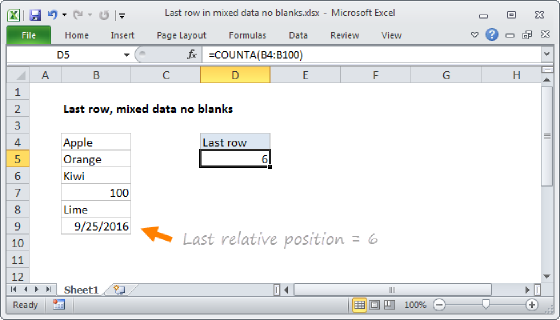
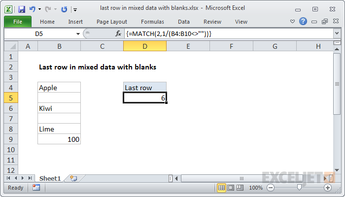
To get the last relative position (i.e. last row, last column) for mixed data that may contain empty cells, you can use the MATCH function as described below.

Note: this is an array formula and must be entered with Control+Shift+Enter.

In the example shown, the formula in E5 is:

{=MATCH(2,1/(B4:B10<>""))}

Last relative position, not row on worksheet

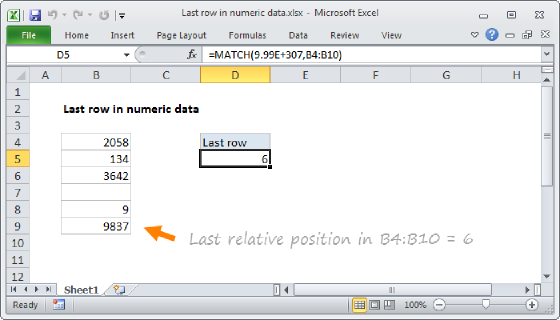
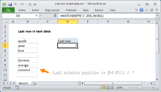
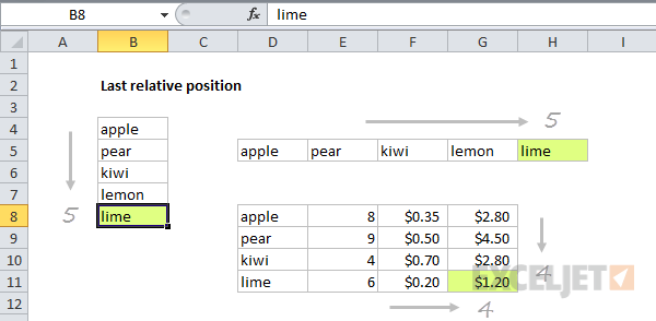
When constructing more advanced formulas, it's often necessary to figure out the last location of data in a list. Depending on the data, this could be the last row with data, the last column with data, or the intersection of both. We want the last *relative position* inside a given range not the row number on the worksheet:

Illustration of last relative position (last row, last column)

Explanation

This formula uses the MATCH function configured to find the position of the last non-empty cell in a range.

Working from the inside out, the lookup array inside MATCH is constructed like this:

=1/(B4:B10<>""))
=1/{TRUE;FALSE;TRUE;FALSE;TRUE;TRUE;FALSE}
={1;#DIV/0!;1;#DIV/0!;1;1;#DIV/0!}

Note: all values in the array are either 1 or the #DIV/0! error.

MATCH is then set to match the value 2 in "approximate match mode", by omitting the 3rd argument is omitted.

Because the lookup value of 2 will never be found, MATCH will always find the last 1 in the lookup array, which corresponds to the last non-empty cell.

This approach will work with any kind of data, including numbers, text, dates, etc. It also works with null text strings that are returned by formulas like this:

=IF(A1<100,"")

Dynamic range

You can use this formula to create a dynamic range with other functions like INDEX and OFFSET. See links below for examples and explanation:

Inspiration for this article came from Mike Girvin's excellent book Control + Shift + Enter, where Mike does a great job explaining the concept of "last relative position".

Author

Dave Bruns

Related formulas

Last row in mixed data with no blanks

This formula uses the COUNTA function to count values in a range. COUNTA counts both numbers and text to so works well with mixed data. The range B4:B8 contains 5 values, so COUNTA returns 5. The number 5 corresponds to the last row (last relative...

Last row in numeric data

This formula uses the MATCH function in approximate match mode to locate the last numeric value in a range. Approximate match enabled by setting by the 3rd argument in MATCH to 1, or omitting this argument, which defaults to 1. The lookup value is a...

Last row in text data

This formula uses the MATCH function in approximate match mode to locate the last text value in a range. Approximate match enabled by setting by the 3rd argument in MATCH to 1, or omitting this argument, which defaults to 1. The lookup value is a so...

Dynamic named range with OFFSET

This formula uses the OFFSET function to generate a range that expands and contracts by adjusting height and width based on a count of non-empty cells. The first argument in OFFSET represents the first cell in the data (the origin), which in this...

Dynamic named range with INDEX

This page shows an example of a dynamic named range created with the INDEX function together with the COUNTA function. Dynamic named ranges automatically expand and contract when data is added or removed. They are an alternative to using an Excel...

Related functions

Excel MATCH Function

MATCH is an Excel function used to locate the position of a lookup value in a row, column, or table. MATCH supports approximate and exact matching, and wildcards (* ?) for partial matches. Often, MATCH is combined...

Excel Formula Training

Formulas are the key to getting things done in Excel. In this accelerated training, you'll learn how to use formulas to manipulate text, work with dates and times, lookup values with VLOOKUP and INDEX & MATCH, count and sum with criteria, dynamically rank values, and create dynamic ranges. You'll also learn how to troubleshoot, trace errors, and fix problems. Instant access. See details here.