Summary
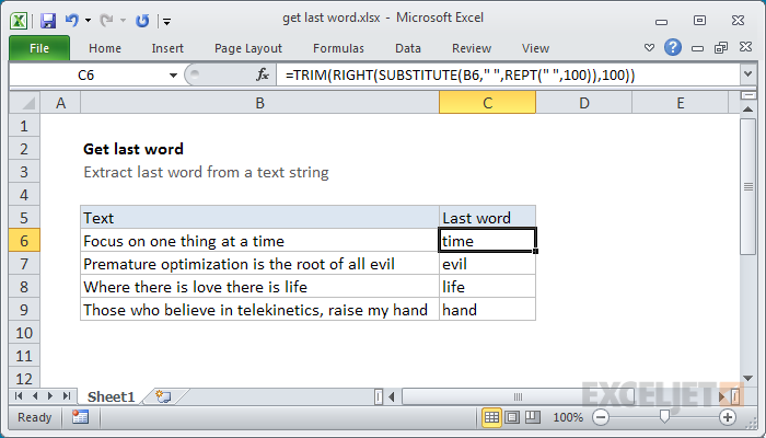
To get the last word from a text string, you can use a formula based on the TRIM, SUBSTITUTE, RIGHT, and REPT functions. In the example shown, the formula in C6 is:
=TRIM(RIGHT(SUBSTITUTE(B6," ",REPT(" ",100)),100))
Which returns the word "time".
Generic formula
=TRIM(RIGHT(SUBSTITUTE(text," ",REPT(" ",100)),100))
Explanation
This formula is an interesting example of a "brute force" approach that takes advantage of the fact that TRIM will remove any number of leading spaces.
Working from the inside out, we use the SUBSTITUTE function to find all spaces in the text, and replace each space with 100 spaces:
SUBSTITUTE(B6," ",REPT(" ",100))
So, for example, with the text string "one two three" the result is going to look like this:
one----------two----------three
With hyphens representing spaces for readability. Keep in mind that there will be 100 spaces between each word.
Next, the RIGHT function extracts 100 characters, starting from the right. The result will look like this:
-------three
Finally, the TRIM function removes all leading spaces, and returns the last word.
Note: We are using 100 arbitrarily because that should be a big enough number to handle very long words. If you have some odd situation with super long words, bump this number up as needed.
Handling inconsistent spacing
If the text you are working with has inconsistent spacing (i.e. extra spaces between words, extra leading or trailing spaces, etc.) This formula won't work correctly. To handle this situation, add an extra TRIM function inside the substitute function like so:
=TRIM(RIGHT(SUBSTITUTE(TRIM(B6)," ",REPT(" ",100)),100))
This will normalize all spaces before the main logic runs.