Details
The Problem
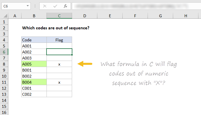
We have a list of alphanumeric codes. Each code consists of a single letter (A, B, C, etc.) followed by a 3-digit number. These codes should appear in alphabetical order, but sometimes they are out of sequence. We want to flag out-of-sequence codes.
Challenge #1
What formula in the "Check" column will place an "x" next to a code that is out of sequence? In this challenge, we are only checking that the *numeric* portion of the code is out of sequence, not that the letter itself is out of sequence.

Challenge #2
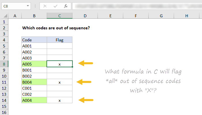
How can the formula above be extended to check if "alpha" part of the code (A,B,C, etc.) is out of sequence? For example, we should flag a code that begins with "A" if it appears after a code that begins with "C" or "B".

Download the worksheet below and take the challenge!
Note: there are 2 sheets in the workbook, one for Challenge #1, one for Challenge #2.
Hint - This video shows some tips for how to solve a problem like this.
Assumptions
- All codes always contain four characters: 1 uppercase letter + 3 numbers.
- The number of codes per letter is random, but there should be no gaps in numeric values.
- It is only necessary to mark the first code with a letter out of sequence, not all subsequent codes.
Here are some working solutions. It's important to understand that there are many, many, ways to solve common problems in Excel. The answers below are just my personal preference. In all of the formulas below, function names are clickable if you want more information.
Challenge #1
I originally went with this formula:
=IF((LEFT(B5)=LEFT(B6))*(MID(B5,2,3)+1<>MID(B6,2,3)+0),"x","")
Note MID returns text. By adding 1 and adding zero, we get Excel to coerce the text into a number. The multiplication inside the logical test inside IF uses boolean logic to avoid another nested IF. I'm not sure why I didn't use RIGHT, which would work fine here as well.
Also note LEFT doesn't require the number of characters and will return the first character if not provided.
Based on some of the clever responses below, we can optimize a bit more:
=IF((LEFT(B5)=LEFT(B6))*(MID(B6,2,3)-MID(B5,2,3)<>1),"x","")
Here, the math operation of subtracting MID from MID automatically coerces the text values to numbers.
Challenge #2
For this solution, I used several nested IFs (line breaks added for readability):
=IF(LEFT(B5)=LEFT(B6),
IF((MID(B5,2,3)+1<>MID(B6,2,3)+0),"x",""),
IF(CODE(B5)+1<>CODE(B6),"x",""))
I did this because the first test LEFT(B5)=LEFT(B6) determines whether we are checking numbers or letters. If the first character is the same, we are checking numbers as above. If not, we are checking the first letter only.
Note the CODE function will return the ascii number of the first character if a text string contains more than 1 character. This feels like a hack, and it makes the code less understandable perhaps, but it works :)
If that offends your sensibilities, use LEFT as above inside CODE to deliver just the first character.


