Native checkboxes in Excel

One of the big changes to Excel in the last year was the introduction of a native checkbox in Excel. Checkboxes might seem like a small thing, but they're very useful for organizing information, tracking progress, and creating interactive spreadsheets. There's something very satisfying about ticking a box to finish off a task!

Unlike the clunky solutions of the past, this new checkbox sits happily in a cell and is very easy to set up. Because the checkbox lives in the grid, it will move around naturally as columns and rows are adjusted. Because it returns TRUE or FALSE, you can use the output directly in formulas and to apply conditional formatting. This means that checkboxes are a great tool to make a spreadsheet interactive.

This article introduces the new native checkbox feature in Excel and walks through a number of practical examples. The examples are all in the attached workbook above, so download the workbook, follow along, and try these new checkboxes out yourself.

Note: this guide is for Excel 365, Excel 2024, and future versions of Excel that have the native checkbox feature. In older versions of Excel, the process for adding a checkbox is different and more complicated.

Table of contents

• The old days: before native checkboxes
• Key features of native checkboxes in Excel
• How to add a checkbox
• How to remove a checkbox
• Checking and unchecking a checkbox
• Example 1: Simple Checklist
• Example 2: Highlight rows with a checkbox
• Example 3: Count and sum checkboxes
• Example 4: Change formula output with a checkbox
• Example 5: Filter a list with a checkbox
• Other important information

The old days: Before native checkboxes

Until Microsoft added the native, in-cell checkbox in 2024, every "checkbox" in Excel was actually a small shape that floated above the grid. To create a checkbox, you first had to show the Developer tab (hidden by default), choose either a Form-control checkbox or an ActiveX checkbox, drop it onto the sheet, and then link it to a cell so formulas could pick up its TRUE/FALSE value. The boxes didn't automatically resize or move if you changed row heights or column widths, and they were easy to misalign or delete.

As a result, most people didn't use checkboxes but instead worked around the problem, using "x" to mark items, showing green ticks with conditional formatting, or creating dropdown lists with "Yes" and "No" options. These solutions work fine, but they aren't elegant or intuitive.

The new checkbox lives inside the cell itself, fills down like ordinary data, survives sorting and filtering, and works consistently on Windows, Mac, web, and mobile. In short, it works like you would expect it to. It's a real upgrade in usability and a great addition to Excel.

Key features of native checkboxes in Excel

The new native checkbox feature is a useful new addition to your day-to-day work in Excel. It's easy to use, with a number of useful features:

• A simple way to mark a task as completed.
• One-step process: Ribbon > Insert > Checkbox.
• User-friendly. No need for form controls or developer tools.
• Native in the Excel grid (no floating objects).
• Compatible with Excel formulas and conditional formatting.
• A nice way to make spreadsheets more interactive and intuitive.
• Cross-platform compatibility. Works on Windows, Mac, and Excel online.

How to add a checkbox

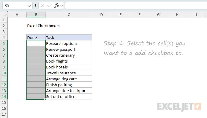
Adding a native checkbox in Excel is easy. First, select the cell(s) you want to add the checkbox to:

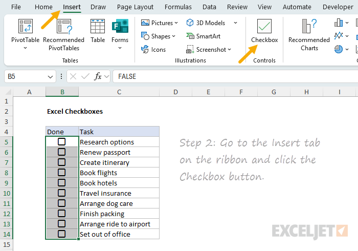
Next, click the Checkbox button on the Insert tab of the ribbon:

That's it! You've added an interactive checkbox to your cell. You can now click the checkbox to toggle between checked and unchecked as you like:

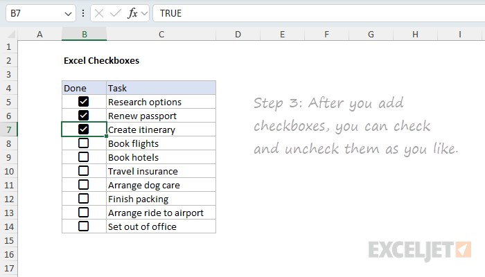
Notice the checkbox will show TRUE (checked) or FALSE (unchecked) in the formula bar as you interact with it.

How to remove a checkbox

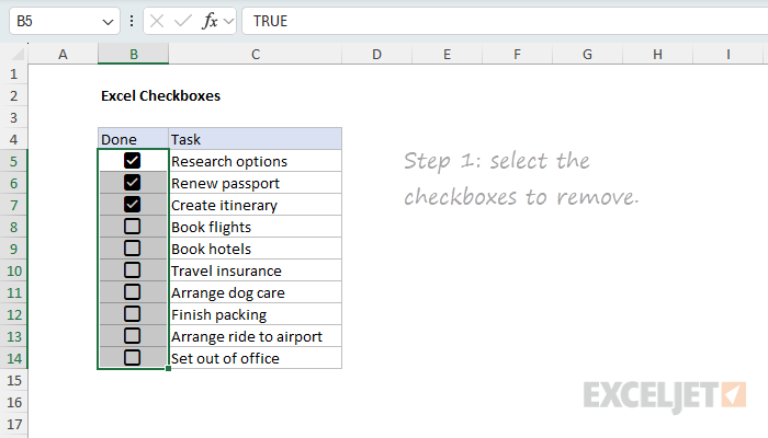
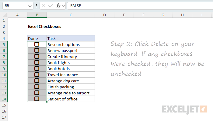
The process to remove a checkbox is also very easy. First, select the cells you want to remove the checkbox from:

Next, click the Delete key on your keyboard. If a checkbox was checked, it will now be unchecked:

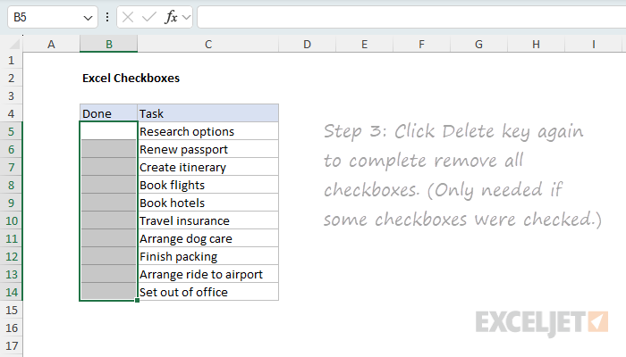
Click the Delete key a second time to completely remove the checkbox:

Checking and unchecking a checkbox

An Excel checkbox is a control that toggles between checked and unchecked. Click once to check it, and click again to uncheck it. If you have more than one checkbox selected, only the first checkbox will be affected.

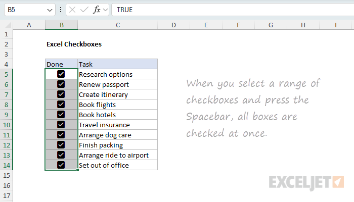
Another way to check and uncheck checkboxes is to use the Spacebar. Press the Spacebar once to check the checkbox, and press it again to uncheck it. A big advantage of the spacebar is that you can use it to check and uncheck all checkboxes in a selection.

First, select the range of checkboxes you want to check or uncheck, then press the Spacebar to check all the checkboxes at once:

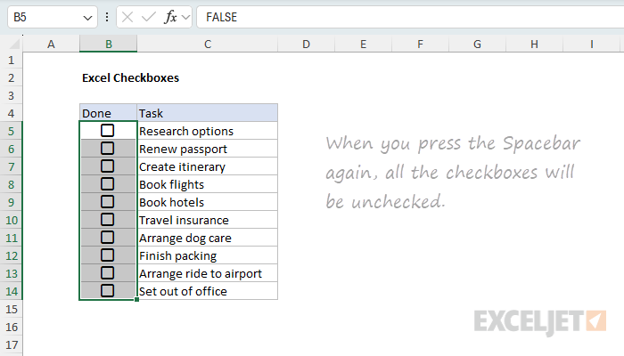
If you press the Spacebar again, all the checkboxes will be unchecked:

The Spacebar behavior changes if any checkboxes are already checked. If checkboxes in the selection are checked, pressing the Spacebar will uncheck them. Press the Spacebar again to check all checkboxes in the selection.

Example 1: Simple Checklist

A classic use of checkboxes is to create a checklist, useful for tracking the completion of tasks or steps. To create a checklist like this, follow the steps explained above:

1. Select the cell(s) you want to add the checkbox to.
2. Click the checkbox button on the Insert tab of the ribbon.
3. Click the checkbox to toggle between checked and unchecked.

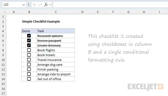
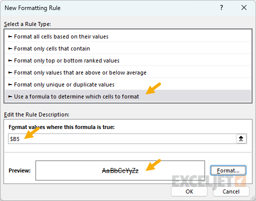
To add a strikethrough effect to the text when the checkbox is checked, use Conditional Formatting. Here are the steps:

1. Select the cells you want to format, C5:C14 in this example.
2. Navigate to Home > Conditional Formatting > New Rule.
3. Select "Use a formula to determine which cells to format" option.
4. Enter the formula =$B5 in the formula bar.
5. Click the Format button and check the "Strikethrough" option.
6. Click OK to save and apply the strikethrough effect.

The screenshot below shows how the rule is configured after adding the formula and setting the strikethrough formatting:

Note: Because checkboxes return TRUE and FALSE, the formula in the conditional formatting rule is simply =$B5. If you prefer, you can use =$B5=TRUE instead. Also, it's not strictly necessary to lock the column reference, but it's useful when you want to copy the rule to other columns.

If you are new to the concept of applying a conditional formatting rule with a formula, watch this short video: How to apply conditional formatting with a formula.

Example 2: Highlight rows with a checkbox

Another useful way to use checkboxes is to highlight rows of interest, as seen in the worksheet below:

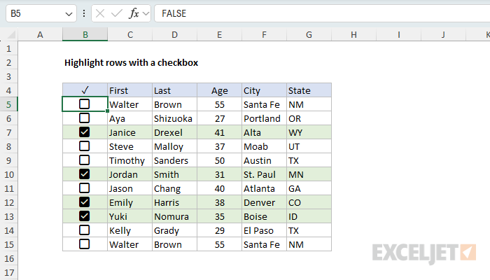
Like the previous example, the formatting is applied using Conditional Formatting. Here are the steps:

1. Select the cells you want to format, B5:G15 in this example.
2. Navigate to Home > Conditional Formattings > New Rule.
3. Select "Use a formula to determine which cells to format" option.
4. Enter the formula =$B5 in the formula bar.
5. Click the Format button and set a Fill color
6. Click OK to save and apply the highlight effect.

The screenshot below shows how the rule is configured after adding the formula and setting the fill color:

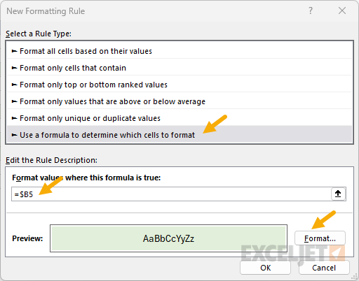
Note: This is a case where we need the mixed reference =$B5 to lock the column and so that it does not change as it is evaluated across all six columns

Example 3: Count and sum checkboxes

Once you are using checkboxes in a worksheet, you may want to count or sum the number of checkboxes that are checked, or sum the values associated with checked or unchecked checkboxes. You can easily do this with the COUNTIFS function and SUMIFS function as shown in the worksheet below:

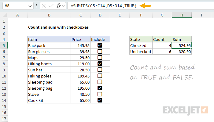
The formulas in column G are set up to count the number of checkboxes that are checked or unchecked D5:D14 using COUNTIFS. The formulas in column H are set up to sum the values in C5:C14 for the checkboxes that are checked or unchecked in D5:D14 using SUMIFS.

G5: =COUNTIFS(D5:D14,TRUE)
G6: =COUNTIFS(D5:D14,FALSE)
H5: =SUMIFS(C5:C14,D5:D14,TRUE)
H6: =SUMIFS(C5:C14,D5:D14,FALSE)

Note that for criteria, we simply use TRUE or FALSE, which is the result of the checkbox.

Example 4: Change formula output with a checkbox

Because checkboxes return TRUE or FALSE, you can use them to change the output of a formula. For example, you can use the result from a checkbox with the IF function to apply a discount or penalty to a value based on whether the checkbox is checked or unchecked. You can see an example of this in the worksheet below, where a checkbox in column D is used to apply a 20% discount to the Price in column C:

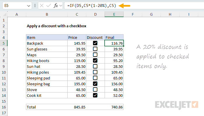
The formula in column E looks like this:

=IF(D5,C5*(1-20%),C5)

Inside the IF function, the logical test is D5, which is the result of the checkbox. If the checkbox is checked, the formula returns C5*(1-20%), which is the price minus 20%. If the checkbox is unchecked, the formula returns C5, which is the original price.

Note: Applying a discount is just one example of how you can use checkboxes to change the output of a formula. Because checkboxes return TRUE or FALSE, you can use them to change the output of almost any formula.

Example 5: Filter a list with a checkbox

Another useful way to use checkboxes is to filter a list based on the checkbox status. You can see an example of this in the worksheet below, where a checkbox in column B (RSVP) is used to filter names in column C with the FILTER function:

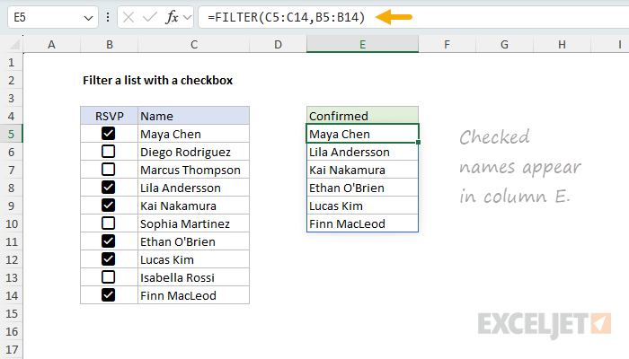
The idea is to create a list of names that have RSVP'd "Yes" to an event. The formula in cell E5 looks like this:

=FILTER(C5:C14,B5:B14)

Inside the FILTER function, the array is given as C5:C14, which is the range of names to filter. The include argument is B5:B14, which is the range of checkboxes to filter by. Because checkboxes return TRUE or FALSE, the result from FILTER is a list of names in column C where RSVP is TRUE (checked).

Other important information

Here are a few other things you should know about using new native checkboxes in Excel:

• Checkboxes are a little like number formatting in that you can copy and paste checkbox formatting using Paste Special > Formats on top of TRUE and FALSE values, and the checkboxes will display correctly. However, if you select a checkbox and examine the Checkbox button on the Insert tab of the ribbon, there is no indication that checkbox formatting has been "applied".
• If you want to turn off the display of checkboxes but keep the TRUE and FALSE values intact, first copy the checkboxes to another location using Paste Special > Values, then turn off the checkboxes and copy and paste the TRUE values back into place. Maybe there's a better way to do this? Let me know if so.
• If you have existing formulas that return TRUE and FALSE, and you insert checkboxes on top of these formulas, the checkboxes will appear correctly. However, checkboxes applied to formulas are read-only; you can't change the state by clicking. The formula underneath the checkbox is the only mechanism that will check and uncheck the box.