Summary
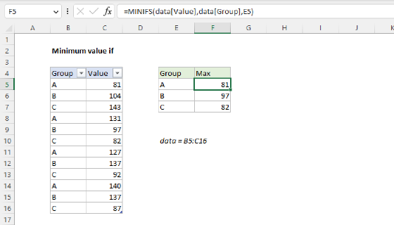
To get the max value if a condition is true, you can use the MAXIFS function. In the example shown, the formula in cell F5 is:
=MAXIFS(data[Value],data[Group],E5)
Where data is an Excel Table in the range B5:C16. As the formula is copied down, the result is the maximum value for each group listed in column E. There are several ways to approach this problem. See below for other formula options, including an all-in-one formula that creates a dynamic summary table.
Generic formula
=MAXIFS(data,range,criteria)
Explanation
In this example, the goal is to get the maximum value for each group in the data as shown. The easiest way to solve this problem is with the MAXIFS function. However, there are actually several options. If you need more flexibility (i.e. you need to work with arrays and not ranges), you can use the MAX function with the FILTER function. To create a dynamic summary table with a single all-in-one formula, you can use the BYROW function. In older versions of Excel without the MAXIFS function, you can use an array formula based on the MAX function and the IF function. Each approach is explained below.
Excel Table
For convenience, all data is in an Excel Table named data in the range B5:C16. Excel Tables are a convenient way to work with data in Excel because they (1) automatically expand to include new data and (2) offer structured references, which allow you to refer to columns by name instead of by address. If you are new to Excel Tables, this article provides an overview.
Video: How to create an Excel Table
MAXIFS function
The MAXIFS function can get the maximum value in a range based on one or more criteria. The generic syntax for MAXIFS with a single condition looks like this:
=MAXIFS(max_range,range1,criteria1)
Note that the condition is defined with two arguments: range1 and criteria1. In this problem, the condition is that the group value in column B must equal the group value in column E. We start off with the max_range, which is the Value column:
=MAXIFS(data[Value],
Next, we add the criteria range, which is the Group column:
=MAXIFS(data[Value],data[Group],
Finally, we add the criteria itself, the value in cell E5:
=MAXIFS(data[Value],data[Group],E5)
As the formula is copied down, the table references behave like absolute references and don't change. The reference to E5 is relative and changes at each new row. The result is the maximum value for each group listed in column E.
The MAXIFS function is a straightforward solution that works well. However, it does have one significant limitation: the range arguments inside MAXIFS must be actual ranges, you can't substitute arrays. If you need to use arrays, see the MAX + FILTER option, or the all-in-one summary table formula based on the BYROW function below.
MAX + FILTER
In the dynamic array version of Excel, another way to solve this problem is with the MAX function and the FILTER function like this:
=MAX(FILTER(data[Value],data[Group]=E5))
Inside the MAX function, the FILTER function is configured to filter values by group:
FILTER(data[Value],data[Group]=E5)
Array is provided as the Value column in the table, and the include argument is a simple expression:
data[Group]=E5
With "A" in cell E5, the expression above returns an array like this:
{TRUE;FALSE;FALSE;TRUE;FALSE;FALSE;TRUE;FALSE;FALSE;TRUE;FALSE;FALSE}
Because there are 12 values in Group, there are 12 TRUE and FALSE results. The TRUE values correspond to values in the table associated with group A. With the array above acting as a filter, the FILTER function returns an array that contains the four values in group A directly to the MAX function:
=MAX({81;131;127;140})
MAX then returns a final result of 140. The primary advantage of using the MAX function with the FILTER function is that you are not required to supply a range of values on the worksheet. You can instead provide an array of values created with another operation. This is very useful when the source data needs to be manipulated in some way before a max value is calculated.
Summary table with BYROW
In the latest version of Excel, which supports dynamic array formulas, you can create a single all-in-one formula that builds the entire summary table, including headers, like this:
=LET(
groups,data[Group],
values,data[Value],
ugroups,UNIQUE(groups),
results,BYROW(ugroups,LAMBDA(r,MAX(FILTER(values,groups=r)))),
VSTACK({"Group","Max"},HSTACK(ugroups, results))
)
The LET function is used to assign four intermediate variables: groups, values, ugroups, and results. Both groups and values are simple assignments to rows in the table:
groups,data[Group],
values,data[Value],
This is done primarily to make the formula more portable. Defining these variables here keeps all of the worksheet references at the top of the formula where they can be easily changed.
In our summary table, we want a list of unique groups, so we define ugroups (unique groups) with the UNIQUE function like this:
ugroups,UNIQUE(groups), // get unique groups
From the 12 rows in the data, the UNIQUE function returns just 3 unique groups:
{"A";"B";"C"} // unique groups
Note: you could run groups through the SORT function to ensure that groups are in the correct order. In this case the source data already shows groups in order, so it is not necessary.
At this point, we are ready to calculate the max values for each group. We do this with the BYROW function which calculates the maximum values and assigns the result to the variable results:
results,BYROW(ugroups,LAMBDA(r,MAX(FILTER(values,groups=r))))
BYROW runs through the ugroups values row by row. At each row, it applies this calculation:
LAMBDA(r,MAX(FILTER(values,groups=r)))
The value r is the unique group in the "current" row in the summary table. Inside the MAX function, the FILTER function is configured to filter values by group like this:
FILTER(values,groups=r)
In the first row (group A), the result from FILTER is an array like this:
{81;131;127;140}
This array is delivered directly to the MAX function, which returns the maximum number. When BYROW is finished, we have an array with 3 numbers (one for each group) like this:
{140;137;143} // results
This array is the value assigned to results. Finally the HSTACK and VSTACK functions are used to assemble a complete table:
VSTACK({"Group","Max"},HSTACK(ugroups, results))
At the top of the table, the array constant {"Group","Max"} creates a header row. The HSTACK function combines ugroups and results horizontally, and VSTACK combines the header row and the data to make the final table. The final result spills into multiple cells on the worksheet.
MAX + IF
In older versions of Excel that do not have the MAXIFS function, you can solve this problem with an array formula based on the MAX function and the IF function like this:
=MAX(IF(data[Group]=E5,data[Value]))
Note: this is an array formula and must be entered with control + shift + enter in Legacy Excel.
Working from the inside out, the IF function is evaluated first. The logical test is an expression that tests the entire Group column against the value in cell E5:
=IF(data[Group]=E5 // logical test
Because there are 12 values in data[Group], the result is an array with 12 TRUE / FALSE values like this:
{TRUE;FALSE;FALSE;TRUE;FALSE;FALSE;TRUE;FALSE;FALSE;TRUE;FALSE;FALSE}
The TRUE values correspond to rows where the group is "A". For all other groups, the value is FALSE. For value_if_true, we supply the Value column, and we omit value_if_false altogether:
IF(data[Group]=E5,data[Value])
The final result from IF is an array like this:
{81;FALSE;FALSE;131;FALSE;FALSE;127;FALSE;FALSE;140;FALSE;FALSE}
Looking at the values in this array, you can see that the IF function acts like a filter. Only numbers associated with group "A" make it through the filter, other values are replaced with FALSE. The IF function delivers this array directly to the MAX function:
=MAX({81;FALSE;FALSE;131;FALSE;FALSE;127;FALSE;FALSE;140;FALSE;FALSE})
The MAX function automatically ignores FALSE values and returns the maximum number in the array: 140.