Summary
The easiest way to calculate a count of the longest winning streak is to use the SCAN function with the MAX function. In the example shown, the formula in cell E5 is:
=MAX(SCAN(0,C5:C22,LAMBDA(a,v,IF(v="w",a+1,0))))
The result is 5 — the longest streak of consecutive wins, starting on April 15 and ending on April 25.
Note: SCAN is only available in the latest version of Excel. See below for formulas that will work in older versions of Excel.
Generic formula
=MAX(SCAN(0,array,LAMBDA(a,v,IF(v="w",a+1,0))))
Explanation
In this example, the goal is to calculate a count for the longest winning streak in a set of data. In the worksheet shown, wins ("W") and losses ("L") are recorded in column C, so this means we want to count the longest consecutive series of W's. Although we are specifically counting the longest winning streak in this example, the same approach can be used to count many other things, including:
- Consecutive days of exercise.
- Consecutive days without symptoms.
- Consecutive days practicing a language or skill.
- Consecutive days not drinking, or not smoking.
- Consecutive days without an accident (at a factory for example).
To handle these use cases, you will need to adjust the formulas to work with the data as recorded.
Options
The article below explains four formula solutions:
- A simple solution based on the SCAN function.
- A more robust SCAN-based formula that lists all winning steaks.
- A simple solution based on a helper column for older versions of Excel.
- A legacy array formula based on the FREQUENCY function.
Options #1 and #2 above require a version of Excel with the SCAN function, which is currently Excel 365. Options #3 and #4 will work in older versions of Excel.
Simple SCAN formula
In the current version of Excel with the SCAN function, the simplest way to solve this problem is like this:
=MAX(SCAN(0,C5:C22,LAMBDA(a,v,IF(v="w",a+1,0))))
The SCAN formula may look scary, but it is actually pretty simple. Starting at zero, SCAN runs through the list of results. When it encounters a "w", it adds 1 to a running count. When it encounters any other value, it resets the running count to zero. SCAN returns the full set of running counts to MAX, which returns the maximum number. Let's look at the details.
The SCAN function applies a custom calculation to each item in an array and returns a new array that contains the intermediate values created during the scan. Because SCAN has a mechanism to keep track of intermediate values (an accumulator), it works well for running totals and other calculations that display intermediate results. In this formula, SCAN is configured like this:
SCAN(0,C5:C22,LAMBDA(a,v,IF(v="w",a+1,0)))
Here, the initial_value is provided as zero (0), and the array is given as C5:C22, which contains 18 values like this:
{"L";"W";"W";"L";"L";"L";"W";"W";"W";"W";"W";"L";"L";"L";"W";"L";"W";"W"}
The custom LAMBDA calculation looks like this:
=LAMBDA(a,v,IF(v="w",a+1,0)
When the value (v) is equal to "w", the accumulator (a) is incremented by 1. Otherwise, the accumulator is reset to zero. The output from SCAN looks like this:
{0;1;2;0;0;0;1;2;3;4;5;0;0;0;1;0;1;2}
This array contains 18 numbers which represent the running counts of consecutive wins. Notice the count starts over again at zero when there is a loss. When there are consecutive wins, it increases. The final step in the formula is to extra the maximum value with the MAX function, which is wrapped around SCAN:
=MAX({0;1;2;0;0;0;1;2;3;4;5;0;0;0;1;0;1;2})
The result is 5, which is the longest streak of consecutive wins.
Formula to list all winning streaks
You can also solve this problem with a more advanced SCAN formula that reports all winning streaks at the same time. You can see the result in the worksheet below, where the formula in E5 is:

=LET(
streaks,SCAN(0,C5:C22,LAMBDA(a,v,IF(v="w",a+1,0))),
shifted,VSTACK(DROP(streaks,1),0),
ends,(streaks>0)*(shifted=0),
FILTER(streaks,ends)
)
This formula uses the LET function to define three variables. First, the variable streaks is defined with SCAN like this:
SCAN(0,C5:C22,LAMBDA(a,v,IF(v="w",a+1,0)))
This is the SCAN formula from the first example above, and the result is the same numeric array of winning streaks:
{0;1;2;0;0;0;1;2;3;4;5;0;0;0;1;0;1;2}
Next, the variable shifted is defined like this:
VSTACK(DROP(streaks,1),0)
Here, we "shift" the streaks array up one row by dropping the first row with DROP, then adding a row that contains zero to the end with VSTACK. The result looks like this:
{1;2;0;0;0;1;2;3;4;5;0;0;0;1;0;1;2;0}
The idea here is to make it easy to make it easy to check any value in streaks together with its "next" value. We use the shifted array to create the variable ends like this:
(streaks>0)*(shifted=0)
This expression uses Boolean algebra to check (1) the current value in streaks is greater than zero and (2) the next value is zero. In other words, we are marking the end of winning streaks. The result from the expression above is an array of 1s and 0s like this:
{0;0;1;0;0;0;0;0;0;0;1;0;0;0;1;0;0;1}
If you study the array closely, you can see that the 1s in this array mark the last row of a winning streak. For example, the third item is a 1, because the 2-game winning streak in rows 2 and 3 has ended. In the last step, we generate a list of winning streaks with the FILTER function like this:
FILTER(streaks,ends)
In this step, the ends array is used to filter the streaks array. Because ends marks the end of winning streaks, the result from FILTER are the counts for the four winning streaks in the data:
{2;5;1;2}
Although this formula is more complicated than the first formula above, it is also more flexible. You can wrap the MAX function around FILTER to get the maximum winning streak, display all winning streaks, or sort or filter the list of winning streaks to suit your needs.
Formula based on a helper column
If you are using an older version of Excel that does not offer the SCAN function, or if you just want a simpler and more transparent approach, you can use a helper column. In the screen below, the helper column is column D and the formula in cell D5 is:
=IF(C5="w",SUM(D4,1),0)

As the formula is copied down, it creates a running total of consecutive wins. If the value in column C is "w", the SUM function is used to sum add 1 to the row above. Otherwise, the count is reset to zero.
Note: using the SUM function like this is a clever way to avoid an error when a cell value contains text, since SUM treats text values as zero. With a normal formula like =IF(C5="w", D4+1,0) the result will be #VALUE! if cell C5 contains "W", because the header text in cell D4 will cause an error. Also, note that Excel is not case-sensitive by default, so we are using a lowercase "w" to test values.
Once the helper column is populated, the MAX function is used in cell F5 to return a final result:
=MAX(D5:D22) // returns 5
The result is 5, the longest streak of consecutive wins in the data.
Legacy array formula based on FREQUENCY
This formula only makes sense in an older version of Excel when you don't want to use a helper column. FREQUENCY is one of those quirky functions that turned up in hard-to-solve problems in the past, before dynamic array formulas were introduced. The formula explained below is an array formula that must be entered with Control + Shift + Enter in Excel 2019 and older.
Do you like tricky formulas? If so, you might like this formula based on the FREQUENCY function:
=MAX(FREQUENCY(IF(list,id),IF(list,,id)))
I ran this formula many years ago in a comment on a Chandoo formula challenge page. Since we don't have a list of numeric ids to work with, and since wins and losses are recorded as "W" and "L" instead of TRUE and FALSE, we need to adjust the formula as follows to make it work for the example on this page:
=MAX(FREQUENCY(IF(C5:C22="w",ROW(C5:C22)),IF(C5:C22="w",0,ROW(C5:C22))))
This is a tricky formula to understand. The key idea is that FREQUENCY gathers numbers into "bins". Each bin has an upper limit and holds the count of all numbers in the data set that are less than or equal to the upper limit, and greater than the previous bin number. The formula creates a new bin at the end of each winning streak using the row number of the loss. All other bins are created as zero. The practical effect is a count of consecutive wins in each bin.
Inside FREQUENCY, the data_array is generated with this code:
IF(C5:C22="w",ROW(C5:C22))
The result is an array with 18 items like this:
{FALSE;6;7;FALSE;FALSE;FALSE;11;12;13;14;15;FALSE;FALSE;FALSE;19;FALSE;21;22}
Notice that only wins make it into this array, appearing as column numbers. The losses become FALSE. The bins_array is generated in a similar way like this:
IF(C5:C22="w",0,ROW(C5:C22))
Here the logic is reversed and the result is an array like this:
{5;0;0;8;9;10;0;0;0;0;0;16;17;18;0;20;0;0}
In this array, only the row numbers for the losses survive as non-zero values, and they become the bins that tally wins. The wins are forced to zero and don't collect any numbers from the data array, since zero or FALSE values are ignored. The final arrays delivered to FREQUENCY look like this:
=FREQUENCY({FALSE;6;7;FALSE;FALSE;FALSE;11;12;13;14;15;FALSE;FALSE;FALSE;19;FALSE;21;22},{5;0;0;8;9;10;0;0;0;0;0;16;17;18;0;20;0;0})
With these inputs, FREQUENCY returns an array of counts per bin that looks like this:
{0;0;0;2;0;0;0;0;0;0;0;5;0;0;0;1;0;0;2}
Finally, the MAX function returns 5, the longest streak of consecutive wins.